1 Introduction
Stability problems for non-autonomous systems are very popular in theoretical researches and applications and are difficult enough even in the deterministic case (see, for instance, [1–3, 6–13, 17]). In this paper via the general method of the Lyapunov functionals construction [14–16] some new multi-condition of stability in probability is obtained for the zero solution of a nonlinear stochastic differential equation with the order of nonlinearity higher than one, with several discrete and distributed delays and time varying coefficients. It is shown that the obtained multi-condition of stability gives for one considered equation at once a set of different complementary of each other sufficient stability conditions. Note that other approaches to analyzing stability in random systems are presented for example in [4, 18].
Consider the scalar nonlinear stochastic differential equation with discrete and distributed delays and time varying coefficients
(1.1)
\[\begin{aligned}{}& dx(t)+\Bigg({\sum \limits_{k=0}^{n}}{a_{k}}(t)x(t-{h_{k}})+{\sum \limits_{k=1}^{n}}{\int _{t-{h_{k}}}^{t}}{b_{k}}(s)x(s)ds+g(t,{x_{t}})\Bigg)dt\\{} & \hspace{1em}+\sigma (t)x(t-\tau )dw(t)=0,\\{} & x(s)=\phi (s)\in {H_{2}},\hspace{2em}s\in [-h,0],\hspace{2em}h=\max [{h_{1}},\dots ,{h_{n}},\tau ],\\{} & |g(t,\varphi )|\le {\int _{-h}^{0}}|\varphi (s){|}^{\alpha }dG(s),\hspace{1em}\alpha >1,\hspace{1em}G={\int _{-h}^{0}}dG(s)<\infty .\end{aligned}\]Here ${a_{k}}(t)$, ${b_{k}}(t)$, $\sigma (t)$ are bounded functions, $w(t)$ is the standard Wiener process on a probability space $\{\varOmega ,\mathfrak{F},\mathbf{P}\}$ [5, 16], ${H_{2}}$ is a space of ${\mathfrak{F}_{0}}$-adapted stochastic processes $\phi (s)$, $s\in [-h,0]$,
\[ \| \phi {\| _{0}}=\underset{s\in [-h,0]}{\sup }|\phi (s)|,\hspace{2em}\| \phi {\| }^{2}=\underset{s\in [-h,0]}{\sup }\mathbf{E}|\phi (s){|}^{2},\]
E is the mathematical expectation, ${h_{0}}=0$, ${h_{k}}>0$, $k=1,\dots ,n$, $\tau \ge 0$, $G(t)$ is a nondecreasing function of bounded variation, the integral with respect to $dG(s)$ is understood in the Stiltjes sense.Definition 1.1.
The zero solution of Equation (1.1) is called:
-
– mean square stable if for each $\varepsilon >0$ there exists a $\delta >0$ such that $\mathbf{E}|x(t,\phi ){|}^{2}<\varepsilon $, $t\ge 0$, provided that $\| \phi {\| }^{2}<\delta $;
-
– exponentially mean square stable if it is mean square stable and there exists $\lambda >0$ such that for each initial function ϕ there exists $C>0$ (which may depend on ϕ) such that $\mathbf{E}|x(t,\phi ){|}^{2}\le C{e}^{-\lambda t}$ for $t>0$;
-
– stable in probability if for any ${\varepsilon _{1}}>0$ and ${\varepsilon _{2}}>0$ there exists $\delta >0$ such that the solution $x(t,\phi )$ of Equation (1.1) satisfies the condition $\mathbf{P}\{{\sup _{t\ge 0}}|x(t,\phi )|>{\varepsilon _{1}}\}<{\varepsilon _{2}}$ for any initial function ϕ such that $\mathbf{P}\{\| \phi {\| _{0}}<\delta \}=1$.
Consider the stochastic differential equation [5]
where $x(t)\in {\mathbf{R}}^{n}$, ${x_{t}}=x(t+s)$, $s\le 0$, ${a_{1}}(t,\varphi )\in {\mathbf{R}}^{n}$, ${a_{2}}(t,\varphi )\in {\mathbf{R}}^{n\times m}$, $w(t)\in {\mathbf{R}}^{m}$, along with some functional $V(t,\varphi ):[0,\infty )\times {H_{2}}\to {\mathbf{R}_{+}}$ that can be presented in the form $V(t,\varphi )=V(t,\varphi (0),\varphi (s))$, $s<0$, and for $\varphi ={x_{t}}$ put
Denote by D the set of functionals, for which the function ${V_{\varphi }}(t,x)$ defined in (1.3) has a continuous derivative with respect to t and second continuous derivative with respect to x. For functionals from D the generator L of Equation (1.2) has the form [5, 16]
(1.4)
\[ \begin{aligned}{}LV(t,{x_{t}})& =\frac{\partial {V_{\varphi }}(t,x(t))}{\partial t}+\nabla {V^{\prime }_{\varphi }}\big(t,x(t)\big){a_{1}}(t,{x_{t}})\\{} & \hspace{1em}+\frac{1}{2}Tr\big[{a^{\prime }_{2}}(t,{x_{t}}){\nabla }^{2}{V_{\varphi }}\big(t,x(t)\big){a_{2}}(t,{x_{t}})\big].\end{aligned}\]If in Equation (1.2) ${a_{1}}(t,0)\equiv 0$, ${a_{2}}(t,0)\equiv 0$ then Equation (1.2) has the zero solution and the following theorems hold.
Theorem 1.1.
Let there exist a functional $V(t,\varphi )\in D$, positive constants ${c_{1}}$, ${c_{2}}$ and the function $\mu (t)$ such that the following conditions hold: $\mu (t)\ge {c_{1}}$ for $t\ge 0$, ${\lim _{t\to \infty }}\mu (t)=\infty $ and
Then the zero solution of Equation (1.2) is asymptotically mean square stable. If, in particular, $\mu (t)={c_{1}}{e}^{\lambda t}$, $\lambda >0$, then the zero solution of Equation (1.2) is exponentially mean square stable.
(1.5)
\[ \mathbf{E}V(t,{x_{t}})\ge \mu (t)\mathbf{E}|x(t){|}^{2},\hspace{2em}\mathbf{E}V(0,\phi )\le {c_{2}}\| \phi {\| }^{2},\hspace{2em}\mathbf{E}LV(t,{x_{t}})\le 0.\]Proof.
Integrating the last inequality in (1.5), we obtain $\mathbf{E}V(t,{x_{t}})\le \mathbf{E}V(0,\phi )$. So,
\[ {c_{1}}\mathbf{E}|x(t){|}^{2}\le \mu (t)\mathbf{E}|x(t){|}^{2}\le \mathbf{E}V(t,{x_{t}})\le \mathbf{E}V(0,\phi )\le {c_{2}}\| \phi {\| }^{2}.\]
It means that the zero solution of (1.2) is mean square stable. Besides, from the inequality $\mathbf{E}|x(t){|}^{2}\le {\mu }^{-1}(t)\mathbf{E}V(0,\phi )$ it follows that the zero solution of (1.2) is asymptotically mean square stable or exponentially mean square stable if $\mu (t)={c_{1}}{e}^{\lambda t}$. The proof is completed. □Theorem 1.2.
[16] Let there exist a functional $V(t,\varphi )\in D$ such that for any solution $x(t)$ of Equation (1.2) the following inequalities hold:
for any initial function ϕ such that $\mathbf{P}(\| \phi {\| _{0}}\le \delta )=1$, where $\delta >0$ is small enough. Then the zero solution of Equation (1.2) is stable in probability.
(1.6)
\[ \begin{array}{c}\displaystyle V(t,{x_{t}})\ge \hspace{0.2778em}{c_{1}}|x(t){|}^{2},\hspace{2em}V(0,\phi )\le \hspace{0.2778em}{c_{2}}\| \phi {\| _{0}^{2}},\\{} \displaystyle LV(t,{x_{t}})\le \hspace{0.2778em}0,\hspace{1em}{c_{1}},{c_{2}}>0,\end{array}\]Via Theorems 1.1, 1.2 a construction of stability conditions for a given stochastic differential equation is reduced to construction of appropriate Lyapunov functionals. Via the general method of the Lyapunov functionals construction [14–16], below some multi-condition of stability in probability for the zero solution of Equation (1.1) is obtained.
2 Exponential mean square stability of the linear equation
In this section sufficient conditions of exponential mean square stability are obtained for the linear part of Equation (1.1), i.e., for Equation (1.1) with $g(t,{x_{t}})\equiv 0$.
Let ${n_{i}}$, $i=1,2$, be integers such that $0\le {n_{i}}\le n$. Put
(2.1)
\[ \begin{aligned}{}S(t)& ={\sum \limits_{k=0}^{{n_{1}}}}{a_{k}}(t\hspace{0.1667em}+\hspace{0.1667em}{h_{k}})\hspace{0.1667em}+{\sum \limits_{k=1}^{{n_{2}}}}{b_{k}}(t){h_{k}},\hspace{1em}\hspace{-0.1667em}{m_{1}}\hspace{0.1667em}=\hspace{0.1667em}\min \{{n_{1}},{n_{2}}\},\hspace{1em}\hspace{-0.1667em}{m_{2}}\hspace{0.1667em}=\hspace{0.1667em}\max \{{n_{1}},{n_{2}}\},\\{} {R_{k}}(t,s)& =\left\{\begin{array}{l@{\hskip10.0pt}l}{a_{k}}(s+{h_{k}})+(s-t+{h_{k}}){b_{k}}(s),& k=1,\dots ,{m_{1}}\\{} {a_{k}}(s+{h_{k}})\hspace{1em}\text{if}\hspace{1em}{n_{1}}>{n_{2}},& k={m_{1}}+1,\dots ,{m_{2}},\\{} (s-t+{h_{k}}){b_{k}}(s)\hspace{1em}\text{if}\hspace{1em}{n_{1}}<{n_{2}},& k={m_{1}}+1,\dots ,{m_{2}},\end{array}\right.\\{} R(t)& ={\sum \limits_{k=1}^{{m_{2}}}}{\int _{t-{h_{k}}}^{t}}|{R_{k}}(t,s)|ds,\hspace{2em}{I_{k}}(i,j)=\left\{\begin{array}{l@{\hskip10.0pt}l@{\hskip10.0pt}l}1& \text{if}& k\in [i,j],\\{} 0& \text{if}& k\notin [i,j],\end{array}\right.\\{} {R_{k}^{\lambda }}(t,s)& =\big(S(t)-\lambda \big){R_{k}}(t,s){I_{k}}(1,{m_{2}})-{b_{k}}(s){I_{k}}({n_{2}}+1,n),\\{} {P_{\lambda }}(t)& =\lambda R(t)+{\sum \limits_{i={n_{1}}+1}^{n}}|{a_{i}}(t)|+{\sum \limits_{i={n_{2}}+1}^{n}}{\int _{t-{h_{i}}}^{t}}|{b_{i}}(\theta )|d\theta ,\\{} {Q_{k}^{\lambda }}(t,s)& =|{R_{k}^{\lambda }}(t,s)|+{P_{\lambda }}(t)|{R_{k}}(t,s)|{I_{k}}(1,{m_{2}})+R(t)|{b_{k}}(s)|{I_{k}}({n_{2}}+1,n),\\{} F(t,\lambda )& =\lambda -2S(t)+{\sum \limits_{k=1}^{n}}\Bigg({\int _{t-{h_{k}}}^{t}}|{R_{k}^{\lambda }}(t,s)|ds+{\int _{t}^{t+{h_{k}}}}{e}^{\lambda {h_{k}}}{Q_{k}^{\lambda }}(\theta ,t)d\theta \Bigg)\\{} & \hspace{1em}+{\sum \limits_{k={n_{1}}+1}^{n}}\big(|{a_{k}}(t)|+{e}^{\lambda {h_{k}}}\big(1+R(t+{h_{k}})\big)|{a_{k}}(t+{h_{k}})|\big)+{e}^{\lambda \tau }{\sigma }^{2}(t+\tau ).\end{aligned}\]By virtue of $S(t)$ and ${R_{k}}(t,s)$ defined in (2.1) Equation (1.1) can be presented in the form of a neutral type stochastic differential equation [16]
where
(2.2)
\[ \begin{aligned}{}dz(t,{x_{t}})& =\Bigg(-S(t)x(t)-{\sum \limits_{k={n_{1}}+1}^{n}}{a_{k}}(t)x(t-{h_{k}})\\{} & \hspace{1em}-{\sum \limits_{k={n_{2}}+1}^{n}}{\underset{t-{h_{k}}}{\overset{t}{\int }}}{b_{k}}(s)x(s)ds-g(t,{x_{t}})\Bigg)dt\\{} & \hspace{1em}-\sigma (t)x(t-\tau )dw(t),\end{aligned}\]Theorem 2.1.
If $g(t,{x_{t}})=0$,
and there exists $\lambda >0$ such that $F(t,\lambda )\le 0$ then the zero solution of Equation (1.1) is exponentially mean square stable.
Proof.
Via (2.4), the zero solution of the auxiliary equation $\dot{y}(t)=-S(t)y(t)$ is exponentially stable and the function $v(t)={e}^{\lambda t}{y}^{2}(t)$, $\lambda >0$, is a Lyapunov function for this equation. Following the procedure of the Lyapunov functionals construction [14–16], we will construct Lyapunov functional V for Equations (2.2), (2.3) in the form $V={V_{1}}+{V_{2}}$, where ${V_{1}}(t,{x_{t}})={e}^{\lambda t}{z}^{2}(t,{x_{t}})$ and the additional functional ${V_{2}}$ will be chosen below. Using (1.4) and (2.2) with $g(t,{x_{t}})=0$, we have
\[\begin{aligned}{}L{V_{1}}(t,{x_{t}})& ={e}^{\lambda t}\Bigg[\lambda {z}^{2}(t,{x_{t}})+{\sigma }^{2}(t){x}^{2}(t-\tau )-2z(t,{x_{t}})\Bigg(S(t)x(t)\\{} & \hspace{1em}+{\sum \limits_{k={n_{1}}+1}^{n}}{a_{k}}(t)x(t-{h_{k}})+{\sum \limits_{k={n_{2}}+1}^{n}}{\int _{t-{h_{k}}}^{t}}{b_{k}}(s)x(s)ds\Bigg)\Bigg].\end{aligned}\]
Calculating and estimating ${z}^{2}(t,{x_{t}})$ via (2.3), (2.1), one can show that
\[\begin{aligned}{}L{V_{1}}(t,{x_{t}})& \le {e}^{\lambda t}\Bigg[\Bigg(\lambda -2S(t)+{\sum \limits_{k=1}^{n}}{\int _{t-{h_{k}}}^{t}}|{R_{k}^{\lambda }}(t,s)|ds+{\sum \limits_{k={n_{1}}+1}^{n}}|{a_{k}}(t)|\Bigg){x}^{2}(t)\\{} & \hspace{1em}+{\sum \limits_{k=1}^{n}}{\int _{t-{h_{k}}}^{t}}{Q_{k}^{\lambda }}(t,s){x}^{2}(s)ds+{\sum \limits_{k={n_{1}}+1}^{n}}\big(1+R(t)\big)|{a_{k}}(t)|{x}^{2}(t-{h_{k}})\\{} & \hspace{1em}+{\sigma }^{2}(t){x}^{2}(t-\tau )\Bigg].\end{aligned}\]
To neutralize the terms with delays in the estimate of $L{V_{1}}$ consider the additional functional
\[\begin{aligned}{}{V_{2}}(t,{x_{t}})& ={\sum \limits_{k=1}^{n}}{\int _{t-{h_{k}}}^{t}}{\int _{t}^{s+{h_{k}}}}{e}^{\lambda (s+{h_{k}})}{Q_{k}^{\lambda }}(\theta ,s){x}^{2}(s)d\theta ds\\{} & \hspace{1em}+{\int _{t-\tau }^{t}}{e}^{\lambda (s+\tau )}{\sigma }^{2}(s+\tau ){x}^{2}(s)ds\\{} & \hspace{1em}+{\sum \limits_{k={n_{1}}+1}^{n}}{\int _{t-{h_{k}}}^{t}}{e}^{\lambda (s+{h_{k}})}\big(1+R(s+{h_{k}})\big)|{a_{k}}(s+{h_{k}})|{x}^{2}(s)ds.\end{aligned}\]
Calculating $L{V_{2}}(t,{x_{t}})$, via (2.1) and $F(t,\lambda )\le 0$ for $V={V_{1}}+{V_{2}}$ we obtain $LV(t,{x_{t}})\le {e}^{\lambda t}F(t,\lambda ){x}^{2}(t)\le 0$. So, the constructed functional $V(t,{x_{t}})$ satisfies Conditions (1.5). Via Theorem 1.1 the zero solution of Equation (1.1) with $g(t,{x_{t}})=0$ is exponentially mean square stable. The proof is completed. □
Corollary 2.1.
If Conditions (2.4), ${\sup _{t\ge 0}}S(t)<\infty $ and
hold then the zero solution of Equation (1.1) is exponentially mean square stable.
(2.5)
\[ \begin{aligned}{}& \underset{t\ge 0}{\sup }\frac{1}{S(t)}\Bigg[{\sum \limits_{k=1}^{n}}\Bigg({\int _{t-{h_{k}}}^{t}}|{R_{k}^{0}}(t,s)|ds+{\int _{t}^{t+{h_{k}}}}{Q_{k}^{0}}(\theta ,t)d\theta \Bigg)\\{} & \hspace{1em}+{\sum \limits_{k={n_{1}}+1}^{n}}\big(|{a_{k}}(t)|+\big(1+R(t+{h_{k}})\big)|{a_{k}}(t+{h_{k}})|\big)+{\sigma }^{2}(t+\tau )\Bigg]<2\end{aligned}\]For the proof it is enough to note that (2.5) is equivalent to the condition ${\sup _{t\ge 0}}F(t,0)<0$ from which it follows that there exists small enough $\lambda >0$ such that the condition $F(t,\lambda )\le 0$ holds too.
3 Stability in probability of the nonlinear equation
In this section it is shown that the sufficient conditions for exponential mean square stability of the linear part of Equation (1.1) also are sufficient conditions for stability in probability of the initial nonlinear equation.
Theorem 3.1.
Let Conditions (2.4) hold and there exist $\lambda >0$ and $\varepsilon >0$ such that
where $F(t,\lambda )$ is defined in (2.1). Then the zero solution of Equation (1.1) is stable in probability.
(3.1)
\[ F(t,\lambda )+{\varepsilon }^{\alpha -1}G\Bigg(1+2{e}^{\lambda h}+{\sum \limits_{k=1}^{{m_{2}}}}{e}^{\lambda {h_{k}}}{\int _{t}^{t+{h_{k}}}}|{R_{k}}(\theta ,t)|d\theta \Bigg)\le 0,\]Proof.
Using the functionals ${V_{1}}$, ${V_{2}}$, defined in the proof of Theorem 2.1, via (2.2), (2.3) we obtain
Note that for $|x(s)|\le \varepsilon $, $s\le t$, via (1.1) and (2.1) we have
and
Substituting (3.3), (3.4) into (3.2), we obtain
(3.2)
\[ \begin{aligned}{}L\big({V_{1}}(t,{x_{t}})+{V_{2}}(t,{x_{t}})\big)& \le {e}^{\lambda t}\Bigg[F(t,\lambda ){x}^{2}(t)-2x(t)g(t,{x_{t}})\\{} & \hspace{1em}+2{\sum \limits_{k=1}^{{m_{2}}}}{\int _{t-{h_{k}}}^{t}}{R_{k}}(t,s)x(s)dsg(t,{x_{t}})\Bigg].\end{aligned}\](3.3)
\[ \begin{aligned}{}2|x(t)g(t,{x_{t}})|& \le 2{\int _{-h}^{0}}|x(t)||x(t+s){|}^{\alpha }dG(s)\\{} & \le {\varepsilon }^{\alpha -1}{\int _{-h}^{0}}\big({x}^{2}(t)+{x}^{2}(t+s)\big)dG(s)\\{} & ={\varepsilon }^{\alpha -1}\Bigg(G{x}^{2}(t)+{\int _{-h}^{0}}{x}^{2}(t+s)dG(s)\Bigg)\end{aligned}\](3.4)
\[ \begin{aligned}{}2\Bigg|& {\sum \limits_{k=1}^{{m_{2}}}}{\int _{t-{h_{k}}}^{t}}{R_{k}}(t,s)x(s)dsg(t,{x_{t}})\Bigg|\\{} & \hspace{1em}\le 2{\sum \limits_{k=1}^{{m_{2}}}}{\int _{t-{h_{k}}}^{t}}{\int _{-h}^{0}}|{R_{k}}(t,s)||x(s)||x(t+\tau ){|}^{\alpha }dsdG(\tau )\\{} & \hspace{1em}\le {\varepsilon }^{\alpha -1}{\sum \limits_{k=1}^{{m_{2}}}}{\int _{t-{h_{k}}}^{t}}{\int _{-h}^{0}}|{R_{k}}(t,s)|\big({x}^{2}(s)+{x}^{2}(t+\tau )\big)dsdG(\tau )\\{} & \hspace{1em}={\varepsilon }^{\alpha -1}\Bigg(G{\sum \limits_{k=1}^{{m_{2}}}}{\int _{t-{h_{k}}}^{t}}|{R_{k}}(t,s)|{x}^{2}(s)ds+R(t){\int _{-h}^{0}}{x}^{2}(t+\tau )dG(\tau )\Bigg).\end{aligned}\]
\[\begin{aligned}{}L\big({V_{1}}(t,{x_{t}})+{V_{2}}(t,{x_{t}})\big)& \le {e}^{\lambda t}\Bigg[F(t,\lambda ){x}^{2}(t)+{\varepsilon }^{\alpha -1}\Bigg(G{x}^{2}(t)\\{} & \hspace{1em}+\big(1+R(t)\big){\int _{-h}^{0}}{x}^{2}(t+\tau )dG(\tau )\\{} & \hspace{1em}+G{\sum \limits_{k=1}^{{m_{2}}}}{\int _{t-{h_{k}}}^{t}}|{R_{k}}(t,s)|{x}^{2}(s)ds\Bigg)\Bigg].\end{aligned}\]
Using the additional functional
\[\begin{aligned}{}{V_{3}}(t,{x_{t}})& ={\varepsilon }^{\alpha -1}\Bigg(2{\int _{-h}^{0}}{\int _{t+s}^{t}}{e}^{\lambda (\tau +h)}{x}^{2}(\tau )d\tau dG(s)\\{} & \hspace{1em}+G{\sum \limits_{k=1}^{{m_{2}}}}{\int _{t-{h_{k}}}^{t}}{\int _{t}^{s+{h_{k}}}}{e}^{\lambda (s+{h_{k}})}|{R_{k}}(\theta ,s)|{x}^{2}(s)d\theta ds\Bigg)\end{aligned}\]
with
\[\begin{aligned}{}L{V_{3}}(t,{x_{t}})& ={\varepsilon }^{\alpha -1}{e}^{\lambda t}\Bigg[2{\int _{-h}^{0}}\big({e}^{\lambda h}{x}^{2}(t)-{e}^{\lambda (s+h)}{x}^{2}(t+s)\big)dG(s)\\{} & \hspace{1em}+G{\sum \limits_{k=1}^{{m_{2}}}}\Bigg({e}^{\lambda {h_{k}}}{\int _{t}^{t+{h_{k}}}}|{R_{k}}(\theta ,t)|d\theta {x}^{2}(t)\\{} & \hspace{1em}-{\int _{t-{h_{k}}}^{t}}{e}^{\lambda (s+{h_{k}}-t)}|{R_{k}}(t,s)|{x}^{2}(s)ds\Bigg)\Bigg],\end{aligned}\]
for the functional $V={V_{1}}+{V_{2}}+{V_{3}}$ via (3.1) we obtain
\[\begin{aligned}{}& LV(t,{x_{t}})\\{} & \hspace{1em}\le {e}^{\lambda t}\Bigg[F(t,\lambda )+{\varepsilon }^{\alpha -1}G\Bigg(1+2{e}^{\lambda h}+{\sum \limits_{k=1}^{{m_{2}}}}{e}^{\lambda {h_{k}}}{\int _{t}^{t+{h_{k}}}}|{R_{k}}(\theta ,t)|d\theta \Bigg)\Bigg]{x}^{2}(t)\\{} & \hspace{1em}\le 0.\end{aligned}\]
So, the constructed functional $V(t,{x_{t}})$ satisfies Conditions (1.6). Via Theorem 1.2 the zero solution of Equation (1.1) is stable in probability. The proof is completed. □For the proof it is enough to note that (2.5) is equivalent to the condition ${\sup _{t\ge 0}}F(t,0)<0$ from which it follows that there exist small enough $\lambda >0$ and $\varepsilon >0$ such that Condition (3.1) holds.
Remark 3.1.
From $0\le {n_{i}}\le n$, $i=1,2$, it follows that the couple (${n_{1}},{n_{2}}$) in Equation (2.2) has ${(n+1)}^{2}$ different values. Thus, Theorem 3.1 generally speaking gives ${(n+1)}^{2}$ different stability conditions at once. Some of these conditions can be infeasible, from some of these conditions can follow some other conditions, the remaining conditions will complement each other.
4 Particular cases of stability condition (2.5)
Following Remark 3.1 let us consider some of possible values of the couple $({n_{1}},{n_{2}})$ and obtain appropriate different stability conditions.
If ${n_{1}}={n_{2}}=0$ then via (2.1) ${m_{1}}={m_{2}}=0$, $S(t)={a_{0}}(t)$, ${R_{k}}(t,s)=0$, $R(t)=0$, ${Q_{k}^{0}}(t,s)=|{R_{k}^{0}}(t,s)|=|{b_{k}}(s)|$, and Condition (2.5) takes the form
If ${n_{1}}=n$, ${n_{2}}=0$ then via (2.1) ${m_{1}}=0$, ${m_{2}}=n$, and Condition (2.5) gives
where
(4.2)
\[ \begin{aligned}{}\underset{t\ge 0}{\sup }\frac{1}{{S_{0}}(t)}& \Bigg[{\sum \limits_{k=1}^{n}}\Bigg({\int _{t-{h_{k}}}^{t}}|{S_{0}}(t){a_{k}}(s+{h_{k}})-{b_{k}}(s)|ds\\{} & +{\int _{t}^{t+{h_{k}}}}|{S_{0}}(\theta ){a_{k}}(t+{h_{k}})-{b_{k}}(t)|d\theta \\{} & +|{b_{k}}(t)|{\int _{t}^{t+{h_{k}}}}{A_{0}}(\theta )d\theta +|{a_{k}}(t+{h_{k}})|{\int _{t}^{t+{h_{k}}}}{B_{0}}(\theta )d\theta \Bigg)\\{} & +{\sigma }^{2}(t+\tau )\Bigg]<2,\end{aligned}\]If ${n_{1}}=0$, ${n_{2}}=n$ then ${m_{1}}=0$, ${m_{2}}=n$, and from Condition (2.5) we obtain
where
where ${S_{2}}(t)={a_{0}}(t)+{\sum _{k=1}^{n}}({a_{k}}(t+{h_{k}})+{b_{k}}(t){h_{k}})$.
(4.3)
\[ \begin{aligned}{}\underset{t\ge 0}{\sup }\Bigg[\frac{1}{{S_{1}}(t)}& \Bigg({\sum \limits_{k=1}^{n}}|{b_{k}}(t)|{\int _{t}^{t+{h_{k}}}}\Bigg({S_{1}}(\theta )+{\sum \limits_{i=1}^{n}}|{a_{i}}(\theta )|\Bigg)(t-\theta +{h_{k}})d\theta \\{} & +{\sum \limits_{k=1}^{n}}\big(|{a_{k}}(t)|+\big(1+{B_{1}}(t+{h_{k}})\big)|{a_{k}}(t+{h_{k}})|\big)+{\sigma }^{2}(t+\tau )\Bigg)\\{} & +{B_{1}}(t)\Bigg]<2,\end{aligned}\]
\[ {S_{1}}(t)={a_{0}}(t)+{\sum \limits_{k=1}^{n}}{b_{k}}(t){h_{k}},\hspace{2em}{B_{1}}(t)={\sum \limits_{k=1}^{n}}{\int _{t-{h_{k}}}^{t}}(s-t+{h_{k}})|{b_{k}}(s)|ds.\]
If at last ${n_{1}}={n_{2}}=n$ then ${m_{1}}={m_{2}}=n$, and Condition (2.5) takes the form
(4.4)
\[ \begin{aligned}{}\underset{t\ge 0}{\sup }& \Bigg[{\sum \limits_{k=1}^{n}}{\int _{t-{h_{k}}}^{t}}|{a_{k}}(s+{h_{k}})+(s-t+{h_{k}}){b_{k}}(s)|ds\\{} & +\frac{1}{{S_{2}}(t)}\Bigg({\sum \limits_{k=1}^{n}}{\int _{t}^{t+{h_{k}}}}{S_{2}}(\theta )|{a_{k}}(t+{h_{k}})+(t-\theta +{h_{k}}){b_{k}}(t)|d\theta \\{} & +{\sigma }^{2}(t+\tau )\Bigg)\Bigg]<2,\end{aligned}\]Using different other combinations of ${n_{1}}$ and ${n_{2}}$, one can get different other stability conditions.
Example 4.1.
To demonstrate a possible connection between the obtained different stability conditions consider, for the sake of simplicity, the equation with constant coefficients and without a non-delay term
For Equation (4.5) $n=1$, so, via Remark 3.1 there are 4 possible stability conditions. Since in Equation (4.5) ${a_{0}}=0$ Condition (4.1) does not hold.
(4.5)
\[ dx(t)+\Bigg(ax(t-h)+b{\int _{t-h}^{t}}x(s)ds+c{x}^{2}(t-h)\Bigg)dt+\sigma x(t-\tau )dw(t)=0.\]Put $p=\frac{1}{2}{\sigma }^{2}$. Condition (4.2) gives $p+|{a}^{2}-b|h+a|b|{h}^{2}<a$ and can be presented in the form
Conditions (4.3) take the form
Calculating the integrals in (4.4) separately for $a\ge 0$ and $a<0$, from Condition (4.4) we obtain
So, if at least one of Conditions (4.6)–(4.8) holds then the zero solution of Equation (4.5) is stable in probability and the zero solution of the linear part ($g(t,{x_{t}})\equiv 0$) of this equation is exponentially mean square stable.
(4.6)
\[ \begin{aligned}{}b& >\frac{p-a(1-ah)}{h(1+ah)}\hspace{1em}\text{if}\hspace{1em}b\le 0,\\{} b& >\frac{p-a(1-ah)}{h(1-ah)}\hspace{1em}\text{if}\hspace{1em}b\in \big(0,{a}^{2}\big),\hspace{1em}0<ah<1,\\{} b& <\frac{a(1+ah)-p}{h(1+ah)}\hspace{1em}\text{if}\hspace{1em}b\ge {a}^{2}.\end{aligned}\](4.8)
\[ p<\left\{\begin{array}{l@{\hskip10.0pt}l@{\hskip10.0pt}l}(a+bh)(1-ah-\frac{1}{2}b{h}^{2})& \text{if}& a\ge 0,\\{} (a+bh)(1-ah-\frac{1}{2}b{h}^{2}-\frac{{a}^{2}}{b})& \text{if}& a<0,\end{array}\right.\hspace{1em}a+bh>0.\]In Fig. 1 stability regions for Equation (4.5), given by Conditions (4.6) (the region (1)), (4.7) (the region (2)) and (4.8) (the region (3)) are shown in the space of the parameters $(a,b)$ for $h=0.5$ and $p=0.2$. Note that the regions (1) and (3) complement of each other but the region (2) is included in the region (3). It means that Condition (4.8) is less conservative than (4.7). Note also that Condition (4.8) coincides with (4.7) for $a=0$ only. In Fig. 2 the similar picture is shown for $h=0.5$ and $p=0.55$.
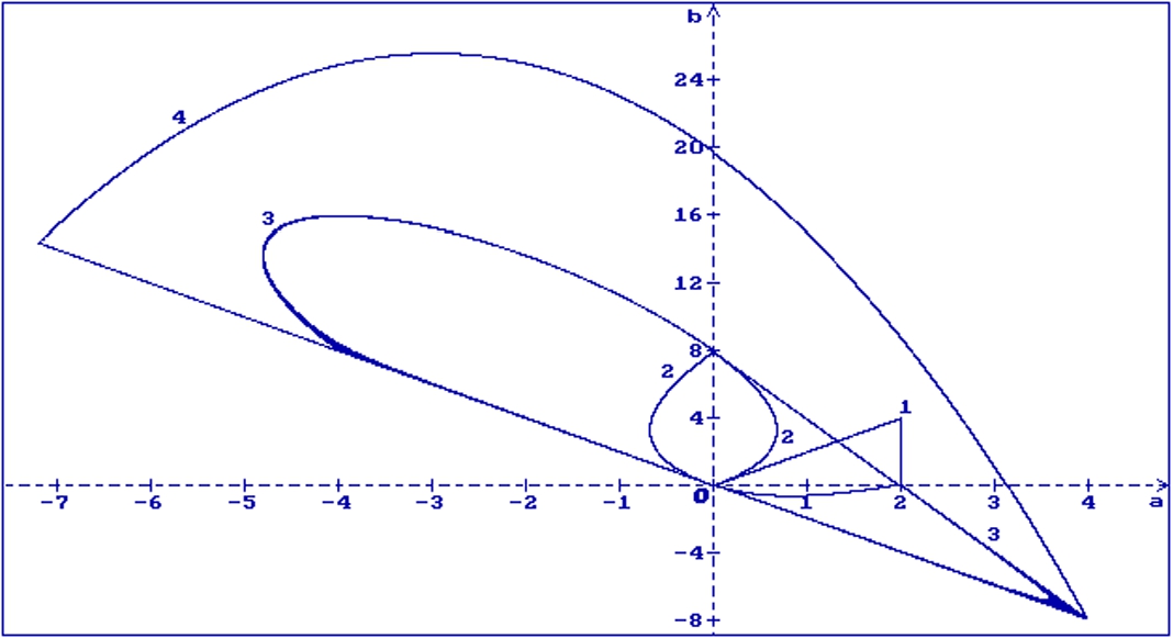
Fig. 3.
Deterministic case ($p=0$) with $h=0.5$. The regions (1), (2), (3) are obtained as in the previous figures, (4) is the exact stability region given by (4.10)
In the deterministic case ($p=0$) the characteristic equation of the linear part of Equation (4.1) has the form
Using $\omega =i\beta $, $i=\sqrt{-1}$, we obtain the system of two algebraic equations for a and b:
In Fig. 3 the stability regions (1), (2), (3) obtained respectively from the sufficient conditions (4.6), (4.7), (4.8) in the deterministic case ($p=0$) are shown for comparison with the exact stability region (4) given by Conditions (4.10) for $h=0.5$. The straight line $a+bh=0$ follows from (4.9) if $\omega \to 0$.
\[ a\cos (h\beta )+\frac{b}{\beta }\sin (h\beta )=0,\hspace{2em}a\sin (h\beta )+\frac{b}{\beta }\big(1-\cos (h\beta )\big)=\beta \]
with the solution
(4.10)
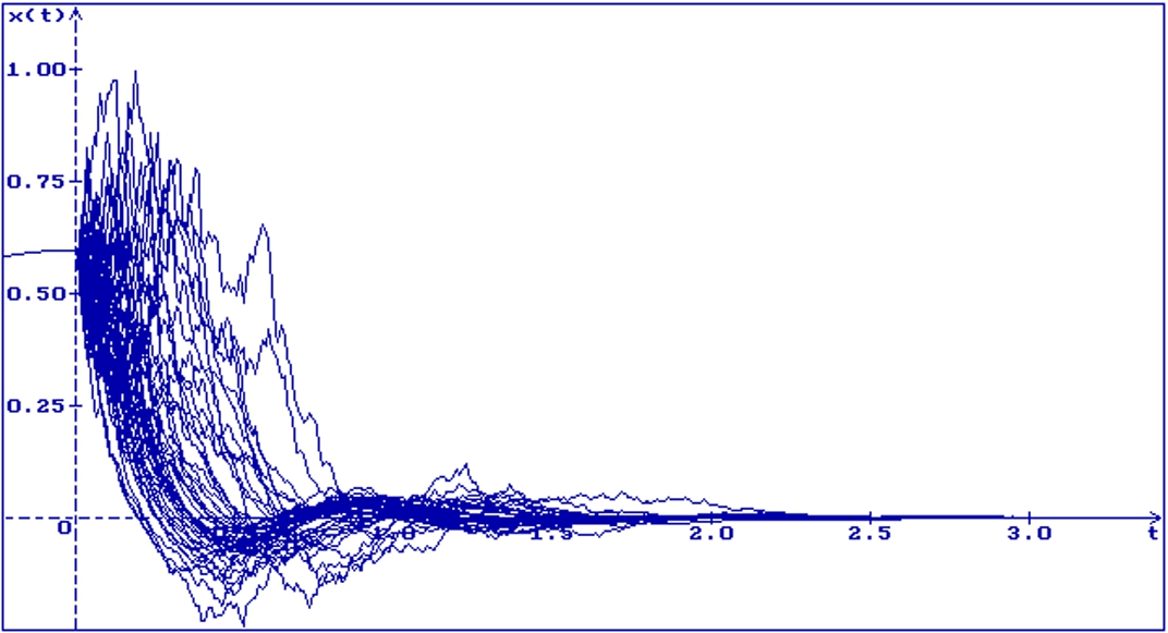
\[ a=\frac{\beta \sin (h\beta )}{1-\cos (h\beta )},\hspace{2em}b=-\frac{{\beta }^{2}\cos (h\beta )}{1-\cos (h\beta )}.\]In Fig. 4, 50 trajectories of the solution of Equation (4.5) are shown at the point $A(-2,9)$ (see Fig. 2) for $c=1$, $h=0.5$, $p=0.55$, $\tau =0$ and the initial function $x(s)=0.6\cos (s)$, $s\in [-h,0]$. The point $A(-2,9)$ is included in the stability region, thus, all trajectories converge to zero.
Remark 4.1.
Suppose that in Equation (1.1) discrete delays are absent, i.e., ${a_{k}}(t)=0$, $k=1,\dots ,n$. Then Conditions (4.2) and (4.4) coincide respectively with (4.1) and (4.3) and are
(4.11)
\[\begin{aligned}{}& \underset{t\ge 0}{\sup }\frac{1}{{a_{0}}(t)}\Bigg[{\sum \limits_{k=1}^{n}}\Bigg(|{b_{k}}(t)|{h_{k}}+{\int _{t-{h_{k}}}^{t}}|{b_{k}}(s)|ds\Bigg)+{\sigma }^{2}(t+\tau )\Bigg]<2,\end{aligned}\](4.12)
\[\begin{aligned}{}& \underset{t\ge 0}{\sup }\Bigg[\frac{1}{{S_{1}}(t)}\Bigg({\sum \limits_{k=1}^{n}}|{b_{k}}(t)|{\int _{t}^{t+{h_{k}}}}{S_{1}}(\theta )(t-\theta +{h_{k}})d\theta +{\sigma }^{2}(t+\tau )\Bigg)+{B_{1}}(t)\Bigg]<2,\\{} & {B_{1}}(t)={\sum \limits_{k=1}^{n}}{\int _{t-{h_{k}}}^{t}}(s-t+{h_{k}})|{b_{k}}(s)|ds,\\{} & {S_{1}}(t)={a_{0}}(t)+{\sum \limits_{k=1}^{n}}{b_{k}}(t){h_{k}}.\end{aligned}\]Example 4.2.
Consider the stochastic differential equation (1.1) with $n=1$, ${a_{0}}(t)=a$, ${h_{1}}=h$, ${b_{1}}(t)=b{e}^{-\mu t}$, $\mu >0$, $\sigma (t)=\sigma {e}^{-\nu t}$, $\nu >0$, $g(t,{x_{t}})=c{x}^{2}(t-h)$, i.e.,
From (4.11) we obtain the first condition for stability in probability of the zero solution of Equation (4.13)
Note that the stability condition (4.14) holds for $a>0$ only. Using (4.12) one can get a complementary condition of stability in probability that holds for $a=0$, $b>0$, $\mu \le 2\nu $. Really, in this case
(4.13)
\[ \begin{aligned}{}& dx(t)+\Bigg(ax(t)+b{\int _{t-h}^{t}}{e}^{-\mu s}x(s)ds+c{x}^{2}(t-h)\Bigg)dt\\{} & \hspace{1em}+\sigma {e}^{-\nu t}x(t-\tau )dw(t)=0.\end{aligned}\](4.14)
\[ \frac{1}{2}|b|\bigg(h+\frac{1}{\mu }\big({e}^{\mu h}-1\big)\bigg)+p{e}^{-2\nu \tau }<a,\hspace{1em}p=\frac{1}{2}{\sigma }^{2}.\]
\[\begin{array}{c}\displaystyle {B_{1}}(t)=\frac{b}{{\mu }^{2}}{e}^{-\mu t}\big({e}^{\mu h}-1-\mu h\big),\hspace{2em}{S_{1}}(t)=bh{e}^{-\mu t},\\{} \displaystyle {\int _{t}^{t+h}}{S_{1}}(\theta )(t-\theta +h)d\theta =\frac{bh}{{\mu }^{2}}{e}^{-\mu t}\big({e}^{-\mu h}-1+\mu h\big),\end{array}\]
and stability condition (4.12) takes the form
\[\begin{array}{c}\displaystyle \underset{t\ge 0}{\sup }\bigg[\frac{b}{{\mu }^{2}}{e}^{-\mu t}\big(\cosh (\mu h)-1\big)+\frac{p}{bh}{e}^{(\mu -2\nu )t}{e}^{-2\nu \tau }\bigg]<1,\\{} \displaystyle \cosh (\mu h)=\frac{1}{2}\big({e}^{\mu h}+{e}^{-\mu h}\big),\hspace{1em}p=\frac{1}{2}{\sigma }^{2}.\end{array}\]
Fig. 4.
50 trajectories of the solution of Equation (4.5), $a=-2$, $b=9$, $c=1$, $h=0.5$, $p=0.55$, $\tau =0$, $x(s)=0.6\cos (s)$, $s\in [-h,0]$
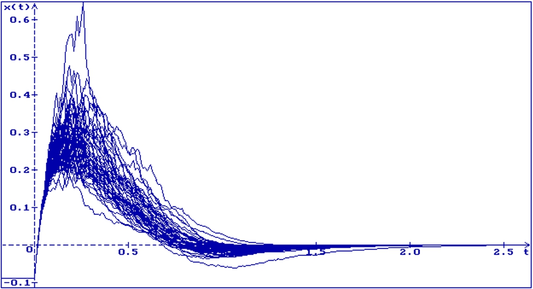
Fig. 5.
50 trajectories of the solution of Equation (4.13), $a=3$, $b=4$, $c=3$, $\mu =0.1$, $\nu =0.01$, $h=0.5$, $p=0.5$, $\tau =0$, $x(s)=-0.09\cos (s)$, $s\in [-h,0]$
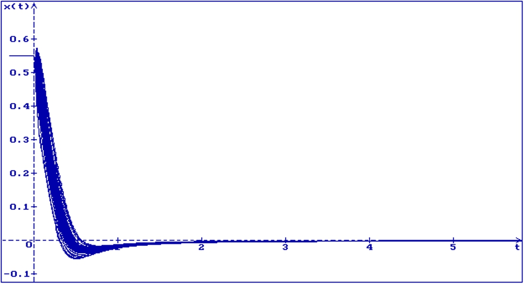
Fig. 6.
50 trajectories of the solution of Equation (4.13), $a=0$, $b=8.5$, $c=1$, $\mu =0.008$, $\nu =0.15$, $h=0.3$, $p=0.2$, $\tau =0$, $x(s)=0.55$, $s\in [-h,0]$
Via $\mu \le 2\nu $, the supremum is reached at $t=0$, so, we obtain $\frac{b}{{\mu }^{2}}(\cosh (\mu h)-1)+\frac{p}{bh}{e}^{-2\nu \tau }<1$ or
So, if one of Conditions (4.14), (4.15) holds then the zero solution of Equation (4.13) is stable in probability.
(4.15)
\[ p<bh\bigg(1-b\frac{\cosh (\mu h)-1}{{\mu }^{2}}\bigg){e}^{2\nu \tau },\hspace{1em}a=0,\hspace{1em}\mu \le 2\nu .\]Note that for $\mu =\nu =0$ Conditions (4.14), (4.15) imply, respectively, two known stability conditions for stochastic differential equations with constant coefficients $a>|b|h+p$ and $bh(1-\frac{b{h}^{2}}{2})>p$ ([16], p. 169).
In Fig. 5, 50 trajectories of the solution of Equation (4.13) are shown for $a=3$, $b=4$, $c=3$, $\mu =0.1$, $\nu =0.01$, $h=0.5$, $p=0.5$, $\tau =0$ and the initial function $x(s)=-0.09\cos (s)$, $s\in [-h,0]$. The stability condition (4.14) holds, thus all trajectories converge to zero. In Fig. 6, 50 trajectories of the solution of Equation (4.13) are shown for $a=0$, $b=8.5$, $c=1$, $\mu =0.008$, $\nu =0.15$, $h=0.3$, $p=0.2$, $\tau =0$ and the initial function $x(s)=0.55$, $s\in [-h,0]$. The stability condition (4.15) holds and all trajectories converge to zero.
5 Conclusions
In this paper, a nonlinear stochastic non-autonomous differential equation with discrete and distributed delays and the order of nonlinearity higher than one is considered. It is shown that investigation of stability in probability of the nonlinear equation of such type can be reduced to investigation of exponential mean square stability of the linear part of the considered equation. A general multi-condition for stability in probability of the zero solution of the considered equation is obtained which allows in applications to get at once a set of different complementary sufficient stability conditions. Some of these conditions can be infeasible, from some of these conditions can follow some other conditions, the remaining conditions will complement each other. The idea of construction of this multi-condition of stability can be used also for systems of nonlinear stochastic differential equations of such type.


