1 Introduction
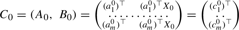
We consider a functional linear error-in-variables model. Let $\{{a_{i}^{0}},\hspace{0.2778em}i\ge 1\}$ be a sequence of unobserved nonrandom n-dimensional vectors. The elements of the vectors are true explanatory variables or (in other terminology) true regressors. We observe m n-dimensional random vectors ${a_{1}},\dots ,{a_{m}}$ and m d-dimensional random vectors ${b_{1}},\dots ,{b_{m}}$. They are thought to be true vectors ${a_{i}^{0}}$ and ${X_{0}^{\top }}{a_{i}^{0}}$, respectively, plus additive errors:
where ${\tilde{a}_{i}}$ and ${\tilde{b}_{i}}$ are random measurement errors in the regressor and in the response. A nonrandom matrix ${X_{0}}$ is estimated based on observations ${a_{i}}$, ${b_{i}}$, $i=1,\dots ,m$.
(1)
\[ \left\{\begin{array}{l}{b_{i}}={X_{0}^{\top }}{a_{i}^{0}}+{\tilde{b}_{i}},\hspace{1em}\\{} {a_{i}}={a_{i}^{0}}+{\tilde{a}_{i}},\hspace{1em}\end{array}\right.\]This problem is related to finding an approximate solution to incompatible linear equations (“overdetermined” linear equation, because the number of equations exceeds the number of variables)
where $A={[{a_{1}},\dots ,{a_{m}}]}^{\top }$ is an $m\times n$ matrix and $B={[{b_{1}},\dots ,{b_{m}}]}^{\top }$ is an $m\times d$ matrix. Here X is an unknown $n\times d$ matrix.
In the linear error-in-variables regression model (1), the Total Least Squares (TLS) estimator in widely used. It is a multivariate equivalent to the orthogonal regression estimator. We are looking for conditions that provide consistency or strong consistency of the estimator. It is assumed (for granted) that the measurement errors ${\tilde{c}_{i}}=(\begin{array}{c}{\tilde{a}_{i}}\\{} {\tilde{b}_{i}}\end{array})$, $i=1,2,\dots $, are independent and have the same covariance matrix Σ. It may be singular. In particular, some of regressors may be observed without errors. (If the matrix Σ is nonsingular, the proofs can be simplified.) An intercept can be introduced into (1) by augmenting the model and inserting a constant error-free regressor.
Sufficient conditions for consistency of the estimator are presented in Gleser [5], Gallo [4], Kukush and Van Huffel [10]. In [18], the consistency results are obtained under less restrictive conditions than in [10]. In particular, there is no requirement that
\[ \frac{{\lambda _{\min }^{2}}({A_{0}^{\top }}{A_{0}})}{{\lambda _{\max }}({A_{0}^{\top }}{A_{0}})}\to \infty \hspace{1em}\text{as}\hspace{1em}m\to \infty ,\]
where ${A_{0}}={[{a_{1}^{0}},\dots ,{a_{m}^{0}}]}^{\top }$ is the matrix A without measurement errors. Hereafter, ${\lambda _{\min }}$ and ${\lambda _{\max }}$ denotes the minimum and maximum eigenvalues of a matrix if all the eigenvalues are real numbers. The matrix ${A_{0}^{\top }}{A_{0}^{}}$ is symmetric (and positive semidefinite). Hence, its eigenvalues are real (and nonnegative).The model where some variables are explanatory and the other are response is called explicit. The alternative is the implicit model, where all the variables are treated equally. In the implicit model, the n-dimensional linear subspace in ${\mathbb{R}}^{n+d}$ is fitted to an observed set of points. Some n-dimensional subspaces can be represented in a form $\{(a,b)\in {\mathbb{R}}^{n+d}:b={X}^{\top }a\}$ for some $n\times d$ matrix X; such subspaces are called generic. The other subspaces are called non-generic. The true points lie on a generic subspace $\{(a,b):b={X_{0}^{\top }}a\}$. A consistently estimated subspace must be generic with high probability. We state our results for the explicit model, but use the ideas of the implicit model in the definition of the estimator, as well as in proofs.
We allow errors in different variables to correlate. Our problem is a minor generalization of the mixed LS-TLS problem, which is studied in [20, Section 3.5]. In the latter problem, some explanatory variables are observed without errors; the other explanatory variables and all the response variables are observed with errors. The errors have the same variance and are uncorrelated. The basic LS model (where the explanatory variables are error-free, and the response variables are error-ridden) and the basic TLS model (where all the variables are observed with error, and the errors are uncorrelated) are marginal cases of the mixed LS-TLS problem. By a linear transformation of variables our model can be transformed into either a mixed LS-TLS or basic LS or basic TLS problem. (We do not handle the case where there are more error-free variables than explanatory variables.) Such a transformation does not always preserve the sets of generic and non-generic subspaces. The mixed LS-TLS problem can be transformed into the basic TLS problem as it is shown in [6].
The Weighted TLS and Structured TLS estimators are generalizations of the TLS estimator for the cases where the error covariance matrices do not coincide for different observations or where the errors for different observations are dependent; more precisely, the independence condition is replaced with the condition on the “structure of the errors”. The consistency of these estimators is proved in Kukush and Van Huffel [10] and Kukush et al. [9]. Relaxing conditions for consistency of the Weighted TLS and Structured TLS estimators is an interesting topic for a future research. For generalizations of the TLS problem, see the monograph [13] and the review [12].
In the present paper, for a multivariate regression model with multiple response variables we consider two versions of the TLS estimator. In these estimators, different norms of the weighted residual matrix are minimized. (These estimators coincide for the univariate regression model.) The common way to construct the estimator is to minimize the Frobenius norm. The estimator that minimizes the Frobenius norm also minimizes the spectral norm. Any estimator that minimizes the spectral norm is consistent under conditions of our consistency theorems (see Theorems 3.5–3.7 in Section 3). We also provide a sufficient condition for uniqueness of the estimator that minimizes the Frobenius norm.
In this paper, for the results on consistency of the TLS estimator which are stated in paper [18], we provide complete and comprehensive proofs and present all necessary auxiliary and complementary results. For convenience of the reader we first present the sketch of proof. Detailed proofs are postponed to the appendix. Moreover, the paper contains new results on the relation between the TLS estimator and the generalized eigenvalue problem.
The structure of the paper is as follows. In Section 2 we introduce the model and define the TLS estimator. The consistency theorems for different moment conditions on the errors and for different senses of consistency are stated in Section 3, and their proofs are sketched in Section 5. Section 4 states the existence and uniqueness of the TLS estimator. Auxiliary theoretical constructions and theorems are presented in Section 6. Section 7 explains the relationship between the TLS estimator and the generalized eigenvalue problem. The results in Section 7 are used in construction of the TLS estimator and in the proof of its uniqueness. Detailed proofs are moved to the appendix (Section 8).
Notations
At first, we list the general notation. For $v\hspace{0.1667em}=\hspace{0.1667em}{({x_{k}})_{k=1}^{n}}$ being a vector, $\| v\| \hspace{0.1667em}=\hspace{0.1667em}\sqrt{{\sum _{k=1}^{n}}{x_{k}^{2}}}$ is the 2-norm of v.
For $M={({x_{i,j}})_{i=1}^{m{_{}^{}}}}$ being an $m\times n$ matrix, $\| M\| ={\max _{v\ne 0}}\frac{\| Mv\| }{\| v\| }={\sigma _{\max }}(M)$ is the spectral norm of M; $\| M{\| _{F}}=\sqrt{{\sum _{i=1}^{m}}{\sum _{j=1}^{n}}{x_{i,j}^{2}}}$ is the Frobenius norm of M; ${\sigma _{\max }}(M)={\sigma _{1}}(M)\ge {\sigma _{2}}(M)\ge \cdots \ge {\sigma _{\min (m,n)}}(M)\ge 0$ are the singular values of M, arranged in descending order; $\operatorname{span}\langle M\rangle $ is the column space of M; $\operatorname{rk}M$ is the rank of M. For a square $n\times n$ matrix M, $\operatorname{def}M=n-\operatorname{rk}M$ is rank deficiency of M; $\operatorname{tr}M={\sum _{i=1}^{n}}{x_{i,i}}$ is the trace of M; ${\chi _{M}}(\lambda )=\det (M-\lambda I)$ is the characteristic polynomial of M. If M is an $n\times n$ matrix with real eigenvalues (e.g., if M is Hermitian or if M admits a decomposition $M=AB$, where A and B are Hermitian matrices, and either A or B is positive semidefinite), ${\lambda _{\min }}(M)={\lambda _{1}}(M)\le {\lambda _{2}}(M)\le \cdots \le {\lambda _{n}}(M)={\lambda _{\max }}(M)$ are eigenvalues of M arranged in ascending order.
For ${V_{1}}$ and ${V_{2}}$ being linear subspaces of ${\mathbb{R}}^{n}$ of equal dimension $\dim {V_{1}}=\dim {V_{2}}$, $\| \sin \angle ({V_{1}},{V_{2}})\| =\| {P_{{V_{1}}}}-{P_{{V_{2}}}}\| =\| {P_{{V_{1}}}}(I-{P_{{V_{2}}}})\| $ is the greatest sine of the canonical angles between ${V_{1}}$ and ${V_{2}}$. See Section 6.2 for more general definitions.
Now, list the model-specific notations. The notations (except for the matrix Σ) come from [9]. The notations are listed here only for reference; they are introduced elsewhere in this paper – in Sections 1 and 2.
n is the number of regressors, i.e., the number of explanatory variables for each observation; d is the number of response variables for each observation; m is the number of observations, i.e., the sample size.
 While in consistency theorems m tends to ∞, all matrices in this list except Σ, ${X_{0}}$ and ${X_{\mathrm{ext}}^{0}}$ silently depend on m. For example, in equations “${\lim _{m\to \infty }}{\lambda _{\min }}({A_{0}^{\top }}{A_{0}})=+\infty $” and “$\widehat{X}\to {X_{0}}$ almost surely” the matrices ${A_{0}}$ and $\widehat{X}$ depend on m.
is the matrix of true variables. It is an $m\times (n+d)$ nonrandom matrix. The left-hand block ${A_{0}}$ of size $m\times n$ consists of true explanatory variables, and the right-hand block ${B_{0}}$ of size $m\times d$ consists of true response variables.
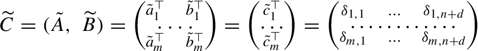
is the matrix of errors. It is an $m\times (n+d)$ random matrix.
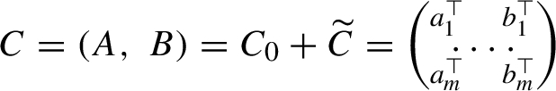
is the matrix of observations. It is an $m\times (n+d)$ random matrix.
Σ
is a covariance matrix of errors for one observation. For every i, it is assumed that $\mathbb{E}{\tilde{c}_{i}}=0$ and $\mathbb{E}{\tilde{c}_{i}}{\tilde{c}_{i}^{\top }}=\varSigma $. The matrix Σ is symmetric, positive semidefinite, nonrandom, and of size $(n+d)\times (n+d)$. It is assumed known when we construct the TLS estimator.
${X_{0}}$
is the matrix of true regression parameters. It is a nonrandom $n\times d$ matrix and is a parameter of interest.
${X_{\mathrm{ext}}^{0}}=\left(\genfrac{}{}{0.0pt}{}{{X_{0}}}{-I}\right)$
is an augmented matrix of regression coefficients. It is a nonrandom $(n+d)\times d$ matrix.
$\widehat{X}$
is the TLS estimator of the matrix ${X_{0}}$.
${\widehat{X}_{\mathrm{ext}}}$
is a matrix whose column space $\operatorname{span}\langle {\widehat{X}_{\mathrm{ext}}}\rangle $ is considered an estimator of the subspace $\operatorname{span}\langle {X_{\mathrm{ext}}^{0}}\rangle $. The matrix ${\widehat{X}_{\mathrm{ext}}}$ is of size $(n+d)\times d$. For fixed m and Σ, ${\widehat{X}_{\mathrm{ext}}}$ is a Borel measurable function of the matrix C.
2 The model and the estimator
2.1 Statistical model
It is assumed that the matrices ${A_{0}}$ and ${B_{0}}$ satisfy the relation
They are observed with measurement errors $\tilde{A}$ and $\widetilde{B}$, that is
The matrix ${X_{0}}$ is a parameter of interest.
(2)
\[ \underset{m\times n}{{A_{0}}}\cdot \underset{n\times d}{{X_{0}}}=\underset{m\times d}{{B_{0}}}.\]Rewrite the relation in an implicit form. Let the $m\times (n+d)$ block matrices ${C_{0}},\widetilde{C},C\in {\mathbb{R}}^{m\times (n+d)}$ be constructed by binding “respective versions” of matrices A and B:
\[ {C_{0}}=[{A_{0}}\hspace{2.5pt}{B_{0}}],\hspace{2em}\widetilde{C}=[\tilde{A}\hspace{2.5pt}\widetilde{B}],\hspace{2em}C=[A\hspace{2.5pt}B].\]
Denote ${X_{\mathrm{ext}}^{0}}=(\begin{array}{c}{X_{0}}\\{} -{I_{d}}\end{array})$. Then
The entries of the matrix $\widetilde{C}$ are denoted ${\delta _{ij}}$; the rows are ${\tilde{c}_{i}}$:
Throughout the paper the following three conditions are assumed to be true:
(4)
\[\begin{aligned}{}& \text{The rows}\hspace{2.5pt}{\tilde{c}_{i}}\hspace{2.5pt}\text{of the matrix}\hspace{2.5pt}\widetilde{C}\hspace{2.5pt}\text{are mutually independent random vectors.}\end{aligned}\](5)
\[\begin{aligned}{}& \mathbb{E}\widetilde{C}=0\text{, and}\hspace{2.5pt}\mathbb{E}{\tilde{c}_{i}^{}}{\tilde{c}_{i}^{\top }}:={(\mathbb{E}{\delta _{ij}}{\delta _{ik}})_{i=1,\hspace{0.1667em}\hspace{0.1667em}k=1}^{n+d\hspace{0.1667em}\hspace{0.1667em}n+d}}=\varSigma \hspace{2.5pt}\text{for all}\hspace{2.5pt}i=1,\dots ,m\text{.}\end{aligned}\]Example 2.1 (simple univariate linear regression with intercept).
For $i=1,\dots ,m$
\[ \left\{\begin{array}{l}{x_{i}}={\xi _{i}}+{\delta _{i}};\hspace{1em}\\{} {y_{i}}={\beta _{0}}+{\beta _{1}}{\xi _{i}}+{\varepsilon _{i}},\hspace{1em}\end{array}\right.\]
where the measurement errors ${\delta _{i}}$, ${\varepsilon _{i}}$, $i=1,\dots ,m$, – all the $2m$ variables – are uncorrelated, $\mathbb{E}{\delta _{i}}=0$, $\mathbb{E}{\delta _{i}^{2}}={\sigma _{\delta }^{2}}$, $\mathbb{E}{\varepsilon _{i}}=0$, and $\mathbb{E}{\varepsilon _{i}^{2}}={\sigma _{\varepsilon }^{2}}$. A sequence $\{({x_{i}},{y_{i}}),\hspace{2.5pt}i=1,\dots ,m\}$ is observed. The parameters ${\beta _{0}}$ and ${\beta _{1}}$ are to be estimated.This example is taken from [1, Section 1.1]. But the notation in Example 2.1 and elsewhere in the paper is different. Our notation is ${a_{i}^{0}}={(1,{\xi _{i}})}^{\top }$, ${b_{i}^{0}}={\eta _{i}}$, ${a_{i}}={(1,{x_{i}})}^{\top }$, ${b_{i}}={y_{i}}$, ${\delta _{i,1}}=0$, ${\delta _{i,2}}={\delta _{i}}$, ${\delta _{i,3}}={\varepsilon _{i}}$, $\varSigma =\operatorname{diag}(0,{\sigma _{\delta }^{2}},{\sigma _{\varepsilon }^{2}})$, and ${X_{0}}={({\beta _{0}},{\beta _{1}})}^{\top }$.
Remark 2.1.
For some matrices Σ, (6) is satisfied for any $n\times d$ matrix ${X_{0}}$. If the matrix Σ in nonsingular, then condition (6) is satisfied. If the errors in the explanatory variables and in the response are uncorrelated, i.e., if the matrix Σ has a block-diagonal form
\[ \varSigma =\left(\begin{array}{c@{\hskip10.0pt}c}{\varSigma _{aa}}& 0\\{} 0& {\varSigma _{bb}}\end{array}\right)\]
(where ${\varSigma _{aa}}=\mathbb{E}{\tilde{a}_{i}}{\tilde{a}_{i}^{\top }}$ and ${\varSigma _{bb}}=\mathbb{E}{\tilde{b}_{i}}{\tilde{b}_{i}^{\top }}$) with nonsingular matrix ${\varSigma _{bb}}$, then condition (6) is satisfied. For example, in the basic mixed LS-TLS problem Σ is diagonal, ${\varSigma _{bb}}$ is nonsingular, and so (6) holds true. If the null-space of the matrix Σ (which equals $\operatorname{span}{\langle \varSigma \rangle }^{\perp }$ because Σ is symmetric) lies inside the subspace spanned by the first n (of $n+d$) standard basis vectors, then condition (6) is also satisfied. On the other hand, if $\operatorname{rk}\varSigma <d$, then condition (6) is not satisfied.2.2 Total least squares (TLS) estimator
First, find the $m\times (n+d)$ matrix Δ for which the constrained minimum is attained
Hereafter ${\varSigma }^{\dagger }$ is the Moore–Penrose pseudoinverse matrix of the matrix Σ, ${P_{\varSigma }}$ is an orthogonal projector onto the column space of Σ, ${P_{\varSigma }}=\varSigma {\varSigma }^{\dagger }$.
(7)
\[ \left\{\begin{array}{l}\| \Delta \hspace{0.1667em}{({\varSigma }^{1/2})}^{\dagger }{\| _{F}}\to \min ;\hspace{1em}\\{} \Delta \hspace{0.1667em}(I-{P_{\varSigma }})=0;\hspace{1em}\\{} \operatorname{rk}(C-\Delta )\le n.\hspace{1em}\end{array}\right.\]Now, show that the minimum in (7) is attained. The constraint $\operatorname{rk}(C-\Delta )\le n$ is satisfied if and only if all the minors of $C-\Delta $ of order $n+1$ vanish. Thus the set of all Δ that satisfy the constraints (the constraint set) is defined by $\frac{m!(n+d)!}{(n+1){!}^{2}(m-n-1)!(d-1)!}+1$ algebraic equations; and so it is closed. The constraint set is nonempty almost surely because it contains $\widetilde{C}$. The functional $\| \Delta {\varSigma }^{\dagger }{\| _{F}}$ is a pseudonorm on ${\mathbb{R}}^{m\times (n+d)}$, but it is a norm on the linear subspace $\{\Delta :\Delta \hspace{0.1667em}(I-{\varSigma }^{\dagger })=0\}$, where it induces a natural subspace topology. The constraint set is closed on the subspace (with the norm), and whenever it is nonempty (i.e., almost surely), it has a minimal-norm element.
Notice that under condition (6) the constrain set is non-empty always and not just almost surely. This follows from Proposition 7.9.
For the matrix Δ that is a solution to minimization problem (7), consider the rowspace $\operatorname{span}\langle {(C-\Delta )}^{\top }\rangle $ of the matrix $C-\Delta $. Its dimension does not exceed n. Its orthogonal basis can be completed to the orthogonal basis in ${\mathbb{R}}^{n+d}$, and the complement consists of $n+d-\operatorname{rk}(C-\Delta )\ge d$ vectors. Choose d vectors from the complement, which are linearly independent, and bind them (as column-vectors) into $(n+d)\times d$ matrix ${\widehat{X}_{\mathrm{ext}}}$. The matrix ${\widehat{X}_{\mathrm{ext}}}$ satisfies the equation
If the lower $d\times d$ block of the matrix ${\widehat{X}_{\mathrm{ext}}}$ is a nonsingular matrix, by linear transformation of columns (i.e., by right-multiplying by some nonsingular matrix) the matrix ${\widehat{X}_{\mathrm{ext}}}$ can be transformed to the form
where I is $d\times d$ identity matrix. The matrix $\widehat{X}$ satisfies the equation
(Otherwise, if the lower block of the matrix ${\widehat{X}_{\mathrm{ext}}}$ is singular, then our estimation fails. Note that whether the lower block of the matrix ${\widehat{X}_{\mathrm{ext}}}$ is singular might depend not only on the observations C, but also on the choice of the matrix Δ where the minimum in (7) in attained and the d vectors that make matrix ${\widehat{X}_{\mathrm{ext}}}$. We will show that the lower block of the matrix ${\widehat{X}_{\mathrm{ext}}}$ is nonsingular with high probability regardless of the choice of Δ and ${\widehat{X}_{\mathrm{ext}}}$.)
Columns of the matrix ${\widehat{X}_{\mathrm{ext}}}$ should span the eigenspace (generalized invariant space) of the matrix pencil $\langle {C}^{\top }C,\varSigma \rangle $ which corresponds to the d smallest generalized eigenvalues. That the columns of the matrix ${\widehat{X}_{\mathrm{ext}}}$ span the generalized invariant space corresponding to finite generalized eigenvalues is written in the matrix notation as follows:
Possible problems that may arise in the course of solving the minimization problem (7) are discussed in [18]. We should mention that our two-step definition $\text{(7)}$ & $\text{(9)}$ of the TLS estimator is slightly different from the conventional definition in [20, Sections 2.3.2 and 3.2] or in [10]. In these papers, the problem from which the estimator $\widehat{X}$ is found is equivalent to the following:
where the optimization is performed for Δ and $\widehat{X}$ that satisfy the constraints in (10). If our estimation defined with (7) and (9) succeeds, then the minimum values in (7) and (10) coincide, and the minimum in (10) is attained for $(\Delta ,\widehat{X})$ that is the solution to (7) & (9). Conversely, if our estimation succeeds for at least one choice of Δ and ${\widehat{X}_{\mathrm{ext}}}$, then all the solutions to (10) can be obtained with different choices of Δ and ${\widehat{X}_{\mathrm{ext}}}$. However, strange things may happen if our estimation always fails.
(10)
\[ \left\{\begin{array}{l}\| \Delta \hspace{0.1667em}{({\varSigma }^{1/2})}^{\dagger }{\| _{F}}\to \min ;\hspace{1em}\\{} \Delta \hspace{0.1667em}(I-{P_{\varSigma }})=0;\hspace{1em}\\{} (C-\Delta )\left(\begin{array}{c}\widehat{X}\\{} -I\end{array}\right)=0,\hspace{1em}\end{array}\right.\]Besides (7), consider the optimization problem
It will be shown that every Δ that minimizes (7) also minimizes (11).
(11)
\[ \left\{\begin{array}{l}{\lambda _{\max }}(\Delta {\varSigma }^{\dagger }{\Delta }^{\top })\to \min ;\hspace{1em}\\{} \Delta \hspace{0.1667em}(I-{P_{\varSigma }})=0;\hspace{1em}\\{} \operatorname{rk}(C-\Delta )\le n.\hspace{1em}\end{array}\right.\]We can construct the optimization problem that generalizes both (7) and (11). Let $\| M{\| _{\mathrm{U}}}$ be a unitarily invariant norm on $m\times (n+d)$ matrices. Consider the optimization problem
Then every Δ that minimizes (7) also minimizes (12), and every Δ that minimizes (12) also minimizes (11). If $\| M{\| _{\mathrm{U}}}$ is the Frobenius norm, then optimization problems (7) and (12) coincide, and if $\| M{\| _{\mathrm{U}}}$ is the spectral norm, then optimization problems (11) and (12) coincide.
(12)
\[ \left\{\begin{array}{l}\| \Delta \hspace{0.1667em}{({\varSigma }^{1/2})}^{\dagger }{\| _{\mathrm{U}}}\to \min ;\hspace{1em}\\{} \Delta \hspace{0.1667em}(I-{P_{\varSigma }})=0;\hspace{1em}\\{} \operatorname{rk}(C-\Delta )\le n.\hspace{1em}\end{array}\right.\]3 Known consistency results
In this section we briefly revise known consistency results. One of conditions for the consistency of the TLS estimator is the convergence of $\frac{1}{m}{A_{0}^{\top }}{A_{0}}$ to a nonsingular matrix. It is required, for example, in [5]. The condition is relaxed in the paper by Gallo [4].
Theorem 3.1 (Gallo [4], Theorem 2).
Let $d=1$,
\[\begin{aligned}{}{m}^{-1/2}{\lambda _{\min }}\big({A_{0}^{\top }}{A_{0}}\big)& \to \infty \hspace{1em}\textit{as}\hspace{1em}m\to \infty ,\\{} \frac{{\lambda _{\min }^{2}}({A_{0}^{\top }}{A_{0}})}{{\lambda _{\max }}({A_{0}^{\top }}{A_{0}})}& \to \infty \hspace{1em}\textit{as}\hspace{1em}m\to \infty ,\end{aligned}\]
and the measurement errors ${\tilde{c}_{i}}$ are identically distributed, with finite fourth moment $\mathbb{E}\| {\tilde{c}_{i}}{\| }^{4}<\infty $. Then $\widehat{X}\stackrel{\mathrm{P}}{\longrightarrow }{X_{0}}$, $m\to \infty $.
The theorem can be generalized for the multivariate regression. The condition that the errors on different observations have the same distribution can be dropped. Instead, Kukush and Van Huffel [10] assume that the fourth moments of the error distributions are bounded.
Theorem 3.2 (Kukush and Van Huffel [10], Theorem 4a).
Let
\[\begin{aligned}{}\underset{\begin{array}{c}i\ge 1\\{} j=1,\dots ,n+d\end{array}}{\sup }\mathbb{E}|{\delta _{ij}}{|}^{4}& <\infty ,\\{} {m}^{-1/2}{\lambda _{\min }}\big({A_{0}^{\top }}{A_{0}}\big)& \to \infty \hspace{1em}\textit{as}\hspace{1em}m\to \infty ,\\{} \frac{{\lambda _{\min }^{2}}({A_{0}^{\top }}{A_{0}})}{{\lambda _{\max }}({A_{0}^{\top }}{A_{0}})}& \to \infty \hspace{1em}\textit{as}\hspace{1em}m\to \infty .\end{aligned}\]
Then $\widehat{X}\stackrel{\mathrm{P}}{\longrightarrow }{X_{0}}$ as $m\to \infty $.
Here is the strong consistency theorem:
Theorem 3.3 (Kukush and Van Huffel [10], Theorem 4b).
Let for some $r\ge 2$ and ${m_{0}}\ge 1$,
\[\begin{aligned}{}\underset{\begin{array}{c}i\ge 1\\{} j=1,\dots ,n+d\end{array}}{\sup }\mathbb{E}|{\delta _{ij}}{|}^{2r}& <\infty ,\\{} {\sum \limits_{m={m_{0}}}^{\infty }}{\bigg(\frac{\sqrt{m}}{{\lambda _{\min }}({A_{0}^{\top }}{A_{0}})}\bigg)}^{r}& <\infty ,\\{} {\sum \limits_{m={m_{0}}}^{\infty }}{\bigg(\frac{{\lambda _{\max }}({A_{0}^{\top }}{A_{0}})}{{\lambda _{\min }^{2}}({A_{0}^{\top }}{A_{0}})}\bigg)}^{r}& <\infty .\end{aligned}\]
Then $\widehat{X}\to {X_{0}}$ as $m\to \infty $, almost surely.
In the following consistency theorem the moment condition imposed on the errors is relaxed.
Theorem 3.4 (Kukush and Van Huffel [10], Theorem 5b).
Let for some r, $1\le r<2$,
\[\begin{aligned}{}\underset{\begin{array}{c}i\ge 1\\{} j=1,\dots ,n+d\end{array}}{\sup }\mathbb{E}|{\delta _{ij}}{|}^{2r}& <\infty ,\\{} {m}^{-1/r}{\lambda _{\min }}\big({A_{0}^{\top }}{A_{0}}\big)& \to \infty \hspace{1em}\textit{as}\hspace{1em}m\to \infty ,\\{} \frac{{\lambda _{\min }^{2}}({A_{0}^{\top }}{A_{0}})}{{\lambda _{\max }}({A_{0}^{\top }}{A_{0}})}& \to \infty \hspace{1em}\textit{as}\hspace{1em}m\to \infty .\end{aligned}\]
Then $\widehat{X}\stackrel{\mathrm{P}}{\longrightarrow }{X_{0}}$ as $m\to \infty $.
Generalizations of Theorems 3.2, 3.3, and 3.4 are obtained in [18]. An essential improvement is achieved. Namely, it is not required that ${\lambda _{\min }^{-2}}({A_{0}^{\top }}{A_{0}}){\lambda _{\max }}({A_{0}^{\top }}{A_{0}})$ converge to 0.
Theorem 3.5 (Shklyar [18], Theorem 4.1, generalization of Theorems 3.2 and 3.4).
Let for some r, $1\le r\le 2$,
\[\begin{aligned}{}\underset{\begin{array}{c}i\ge 1\\{} j=1,\dots ,n+d\end{array}}{\sup }\mathbb{E}|{\delta _{ij}}{|}^{2r}& <\infty ,\\{} {m}^{-1/r}{\lambda _{\min }}\big({A_{0}^{\top }}{A_{0}}\big)& \to \infty \hspace{1em}\textit{as}\hspace{1em}m\to \infty .\end{aligned}\]
Then $\widehat{X}\stackrel{\mathrm{P}}{\longrightarrow }{X_{0}}$ as $m\to \infty $.
Theorem 3.6 (Shklyar [18], Theorem 4.2, generalization of Theorem 3.3).
Let for some $r\ge 2$ and ${m_{0}}\ge 1$,
\[\begin{aligned}{}\underset{\begin{array}{c}i\ge 1\\{} j=1,\dots ,n+d\end{array}}{\sup }\mathbb{E}|{\delta _{ij}}{|}^{2r}& <\infty ,\\{} {\sum \limits_{m={m_{0}}}^{\infty }}{\bigg(\frac{\sqrt{m}}{{\lambda _{\min }}({A_{0}^{\top }}{A_{0}})}\bigg)}^{r}& <\infty .\end{aligned}\]
Then $\widehat{X}\to {X_{0}}$ as $m\to \infty $, almost surely.
In the next theorem strong consistency is obtained for $r<2$.
Theorem 3.7 (Shklyar [18], Theorem 4.3).
Let for some r ($1\le r\le 2$) and ${m_{0}}\ge 1$,
\[ \underset{\begin{array}{c}i\ge 1\\{} j=1,\dots ,n+d\end{array}}{\sup }\mathbb{E}|{\delta _{ij}}{|}^{2r}<\infty ,\hspace{2em}{\sum \limits_{m={m_{0}}}^{\infty }}\frac{1}{{\lambda _{\min }^{r}}({A_{0}^{\top }}{A_{0}})}<\infty .\]
Then $\widehat{X}\to {X_{0}}$ as $m\to \infty $, almost surely.
4 Existence and uniqueness of the estimator
When we speak of sequence $\{{A_{m}},\hspace{0.2778em}m\ge 1\}$ of random events parametrized by sample size m, we say that a random event occurs with high probability if the probability of the event tends to 1 as $m\to \infty $, and we say that a random event occurs eventually if almost surely there exists ${m_{0}}$ such that the random event occurs whenever $m>{m_{0}}$, that is $\mathbb{P}(\underset{m\to \infty }{\liminf }{A_{m}})=1$. (In this definition, ${A_{m}}$ are random events. Elsewhere in this paper, ${A_{m}}$ are matrices.)
Theorem 4.1.
Theorem 4.2.
-
2. Under the conditions of Theorem 3.5, the following random event occurs with high probability: for any Δ that is a solution to (11), equation (9) has a solution $\widehat{X}$. (Equation (9) might have multiple solutions.) The solution is a consistent estimator of ${X_{0}}$, i.e., $\widehat{X}\to {X_{0}}$ in probability.
5 Sketch of the proof of Theorems 3.5–3.7
Denote
Under the conditions of any of the consistency theorems in Section 3 there is a convergence ${\lambda _{\min }}({A_{0}^{\top }}{A_{0}^{}})\to \infty $. Hence the matrix N is nonsingular for m large enough. The matrix N is used as the denominator in the law of large numbers. Also, it is used for rescaling the problem: the condition number of ${N}^{-1/2}{C_{0}^{\top }}{C_{0}^{}}{N}^{-1/2}$ equals 2 at most.
The proofs of consistency theorems differ one from another, but they have the same structure and common parts. First, the law of large numbers
holds either in probability or almost surely, which depends on the theorem being proved. The proof varies for different theorems.
The inequalities (54) and (57) imply that whenever convergence (13) occurs, the sine between vectors ${\widehat{X}_{\mathrm{ext}}}$ and ${X_{\mathrm{ext}}^{0}}$ (in the univariate regression) or the largest of sines of canonical values between column spans of matrices ${\widehat{X}_{\mathrm{ext}}}$ and ${X_{\mathrm{ext}}^{0}}$ tends to 0 as the sample size m increases:
To prove (14), we use some algebra, the fact that ${X_{\mathrm{ext}}^{0}}$ (in the univariate model) or the columns of ${X_{\mathrm{ext}}^{0}}$ (in the multivariate model) are the minimum-eigenvalue eigenvectors of matrix N (see ineq. (52)), and eigenvector perturbation theorems – Lemma 6.5 or Lemma 6.6.
(14)
\[ \big\| \sin \angle ({\widehat{X}_{\mathrm{ext}}},{X_{\mathrm{ext}}^{0}})\big\| \le \big\| \sin \angle \big({N}^{1/2}{\widehat{X}_{\mathrm{ext}}},{N}^{1/2}{X_{\mathrm{ext}}^{0}}\big)\big\| \to 0.\]Then, by Theorem 8.3 we conclude that
6 Relevant classical results
We use some classical results. However, we state them in a form convenient for our study and provide the proof for some of them.
6.1 Generalized eigenvectors and eigenvalues
In this paper we deal with real matrices. Most theorems in this section can be generalized for matrices with complex entries by requiring that matrices be Hermitian rather than symmetric, and by complex conjugating where it is necessary.
Theorem 6.1 (Simultaneous diagonalization of a definite matrix pair).
Let A and B be $n\times n$ symmetric matrices such that for some α and β the matrix $\alpha A+\beta B$ is positive definite. Then there exist a nonsingular matrix T and diagonal matrices Λ and M such that
If in the decomposition $T=[{u_{1}},{u_{2}},\dots ,{u_{n}}]$, $\varLambda =\operatorname{diag}({\lambda _{1}},\dots ,{\lambda _{n}})$, $\mathrm{M}=\operatorname{diag}({\mu _{1}},\dots ,{\mu _{n}})$, then the numbers ${\lambda _{i}}/{\mu _{i}}\in \mathbb{R}\cup \{\infty \}$ are called generalized eigenvalues, and the columns ${u_{i}}$ of the matrix T are called the right generalized eigenvectors of the matrix pencil $\langle A,B\rangle $ because the following relation holds true:
Theorem 6.1 is well known; see Theorem IV.3.5 in [19, page 318]. The conditions of Theorem 6.1 can be changed as follows:
In Theorem 6.1 ${\lambda _{i}}$ and ${\mu _{i}}$ cannot be equal to 0 for the same i, while in Theorem 6.2 they can. On the other hand, in Theorem 6.1 ${\lambda _{i}}$ and ${\mu _{i}}$ can be any real numbers, while in Theorem 6.2 ${\lambda _{i}}\ge 0$ and ${\mu _{i}}\ge 0$. Theorem 6.2 is proved in [15].
Remark 6.2-1.
If the matrices A and B are symmetric and positive semidefinite, then
where
is the determinantal rank of the matrix pencil $\langle A,B\rangle $. (For square $n\times n$ matrices A and B, the determinantal rank characterizes if the matrix pencil is regular or singular. The matrix pencil $\langle A,B\rangle $ is regular if $\operatorname{rk}\langle A,B\rangle =n$, and singular if $\operatorname{rk}\langle A,B\rangle <n$.)
The inequality $\operatorname{rk}\langle A,B\rangle \ge \operatorname{rk}(A+B)$ follows from the definition of the determinantal rank. For all $k\in \mathbb{R}$ and for all such vectors x that $(A+B)x=0$ we have ${x}^{\top }Ax+{x}^{\top }Bx=0$, and because of positive semidefiniteness of matrices A and B, ${x}^{\top }Ax\ge 0$ and ${x}^{\top }Bx\ge 0$. Thus, ${x}^{\top }Ax={x}^{\top }Bx=0$. Again, due to positive semidefiniteness of A and B, $Ax=Bx=0$ and $(A+kB)x=0$. Thus, for all $k\in \mathbb{R}$
\[\begin{aligned}{}\big\{x:(A+B)x=0\big\}& \subset \big\{x:(A+kB)x=0\big\},\\{} \operatorname{rk}(A+B)& \ge \operatorname{rk}(A+kB),\\{} \operatorname{rk}\langle A,B\rangle =\underset{k}{\max }\operatorname{rk}(A+kB)& \le \operatorname{rk}(A+B),\end{aligned}\]
and (17) is proved.Remark 6.2-2.
Let A and B be positive semidefinite matrices of the same size such that $\operatorname{rk}(A+B)=\operatorname{rk}(B)$. The representation (16) might be not unique. But there exists a representation (16) such that
\[\begin{aligned}{}{\lambda _{i}}& ={\mu _{i}}=0\hspace{1em}\text{if}\hspace{1em}i=1,\dots ,\operatorname{def}(B),\\{} {\mu _{i}}& >0\hspace{1em}\text{if}\hspace{1em}i=\operatorname{def}(B)+1,\dots ,n,\\{} T& =\big[\hspace{-0.1667em}\underset{n\times \operatorname{def}(B)}{{T_{1}}}\hspace{0.1667em}\hspace{0.1667em}\underset{n\times \operatorname{rk}(B)}{{T_{2}}}\hspace{-0.1667em}\big],\\{} {T_{1}^{\top }}{T_{2}^{}}& =0.\end{aligned}\]
(Here if the matrix B is nonsingular, then ${T_{1}}$ is $n\times 0$ empty matrix; if $B=0$, then ${T_{2}}$ is $n\times 0$ matrix. In these marginal cases, ${T_{1}^{\top }}{T_{2}}$ is an empty matrix and is considered to be zero matrix.) The desired representation can be obtained from [2] for $S=0$ (in de Leeuw’s notation). This representation is constructed as follows. Let the columns of matrix ${T_{1}}$ make the orthogonal normalized basis of $\operatorname{Ker}(B)=\{v:Bv=0\}$. There exists $n\times \operatorname{rk}(B)$ matrix F such that $B=F{F}^{\top }$. Let the columns of matrix L be the orthogonal normalized eigenvectors of the matrix ${F}^{\dagger }A{({F}^{\dagger })}^{\top }$. Then set ${T_{2}}={({F}^{\dagger })}^{\top }L$. Note that the notation S, F and L is borrowed from [2], and is used only once. Elsewhere in the paper, the matrix F will have a different meaning.Proposition 6.3.
Proof.
Let us verify the Moore–Penrose conditions:
and the fact that the matrices ${({T}^{-1})}^{\top }\text{M}{T}^{-1}\hspace{0.1667em}T{\text{M}}^{\dagger }{T}^{\top }$ and $T{\text{M}}^{\dagger }{T}^{\top }\times {({T}^{-1})}^{\top }\text{M}{T}^{-1}$ are symmetric. The equalities $\text{(18)}$ and $\text{(19)}$ can be verified directly; and the symmetry properties can be reduced to the equality
with ${P_{\mathrm{M}}}=\mathrm{M}{\mathrm{M}}^{\dagger }=\operatorname{diag}(\underset{\operatorname{def}(B)}{\underbrace{0,\dots ,0}},\underset{\operatorname{rk}(B)}{\underbrace{1,\dots ,1}})$.
Since ${T_{1}^{\top }}{T_{2}^{}}=0$, ${T}^{\top }{T}^{}$ is a block diagonal matrix. Hence ${P_{\mathrm{M}}}{T}^{\top }T={T}^{\top }{T}^{}{P_{\mathrm{M}}}$, whence (20) follows. □
6.2 Angle between two linear subspaces
Let ${V_{1}}$ and ${V_{2}}$ be linear subspaces of ${\mathbb{R}}^{n}$, with $\dim {V_{1}}={k_{1}}\le \dim {V_{2}}={k_{2}}$. Then there exists an orthogonal $n\times n$ matrix U such that
Here rectangular diagonal matrices are allowed. If in (21) there are more cosines than sines (i.e., if ${k_{2}}+{k_{1}}>n$), then the excessive cosines should be equal to 1, so the columns of the bidiagonal matrix in (21) are unit vectors (which are orthogonal to each other). Here the columns of U are the vectors of some convenient “new” basis in ${\mathbb{R}}^{n}$, so U is a transitional matrix from the standard basis to “new” basis; the columns of matrix products in $\operatorname{span}\langle \cdots \hspace{0.1667em}\rangle $ in (21) and (22) are the vectors of the bases of subspaces ${V_{1}}$ and ${V_{2}}$; the bidiagonal matrix in (21) and the diagonal matrix in (22) are the transitional matrices from “new” basis in ${\mathbb{R}}^{n}$ to the bases in ${V_{1}}$ and ${V_{2}}$, respectively.
(21)
\[\begin{aligned}{}{V_{1}}& =\operatorname{span}\left\langle U\left(\begin{array}{c}{\operatorname{diag}_{{k_{2}}\times {k_{1}}}}(\cos {\theta _{i}},\hspace{0.2778em}i=1,\dots ,{k_{1}})\\{} {\operatorname{diag}_{(n-{k_{2}})\times {k_{1}}}}(\sin {\theta _{i}},\hspace{0.2778em}i=1,\dots ,\min (n-{k_{2}},\hspace{0.2222em}{k_{1}}))\end{array}\right)\right\rangle ,\end{aligned}\]The angles ${\theta _{k}}$ are called the canonical angles between ${V_{1}}$ and ${V_{2}}$. They can be selected so that $0\le {\theta _{k}}\le \frac{1}{2}\pi $ (to achieve this, we might have to reverse some vectors of the bases).
Denote ${P_{{V_{1}}}}$ the matrix of the orthogonal projector onto ${V_{1}}$. The singular values of the matrix ${P_{{V_{1}}}}(I-{P_{{V_{2}}}})$ are equal to $\sin {\theta _{k}}$ ($k=1,\dots ,{k_{1}}$); besides them, there is a singular value 0 of multiplicity $n-{k_{1}}$.
Denote the greatest of the sines of the canonical eigenvalues
If $\dim {V_{1}}=1$, ${V_{1}}=\operatorname{span}\langle v\rangle $, then
\[ \sin \angle (v,{V_{2}})=\bigg\| (I-{P_{{V_{2}}}})\frac{v}{\| v\| }\bigg\| =\operatorname{dist}\bigg(\frac{1}{\| v\| }v,{V_{2}}\bigg).\]
This can be generalized for $\dim {V_{1}}\ge 1$:
\[ \big\| \sin \angle ({V_{1}},{V_{2}})\big\| =\underset{v\in {V_{1}}\setminus \{0\}}{\max }\bigg\| (I-{P_{{V_{2}}}})\frac{v}{\| v\| }\bigg\| ,\]
whence
(24)
\[\begin{aligned}{}{\big\| \sin \angle ({V_{1}},{V_{2}})\big\| }^{2}& =\underset{v\in {V_{1}}\setminus \{0\}}{\max }\frac{{v}^{\top }(I-{P_{{V_{2}}}})v}{\| v{\| }^{2}},\\{} 1-{\big\| \sin \angle ({V_{1}},{V_{2}})\big\| }^{2}& =\underset{v\in {V_{1}}\setminus \{0\}}{\min }\frac{{v}^{\top }{P_{{V_{2}}}}v}{\| v{\| }^{2}}.\end{aligned}\]If $\dim {V_{1}}=\dim {V_{2}}$, then $\| \sin \angle ({V_{1}},{V_{2}})\| =\| {P_{{V_{1}}}}-{P_{{V_{2}}}}\| $, and therefore $\| \sin \angle ({V_{1}},{V_{2}})\| =\| \sin \angle ({V_{2}},{V_{1}})\| $. Otherwise the right-hand side of (23) may change if ${V_{1}}$ and ${V_{2}}$ are swapped (particularly, if $\dim {V_{1}}<\dim {V_{2}}$, then $\| {P_{{V_{1}}}}(I-{P_{{V_{2}}}})\| $ may or may not be equal to 1, but always $\| {P_{{V_{2}}}}(I-{P_{{V_{1}}}})\| =1$; see the proof of Lemma 8.2 in the appendix).
We will often omit “span” in arguments of sine. Thus, for n-row matrices ${X_{1}}$ and ${X_{2}}$, $\| \sin \angle ({X_{1}},{V_{2}})\| =\| \sin \angle (\operatorname{span}\langle {X_{1}}\rangle ,{V_{2}})\| $ and $\| \sin \angle ({X_{1}},{X_{2}})\| =\| \sin \angle (\operatorname{span}\langle {X_{1}}\rangle ,\operatorname{span}\langle {X_{2}}\rangle )\| $.
Lemma 6.4.
Let ${V_{11}}$, ${V_{2}}$ and ${V_{13}}$ be three linear subspaces in ${\mathbb{R}}^{n}$, with $\dim {V_{11}}={d_{1}}<\dim {V_{2}}={d_{2}}<\dim {V_{13}}={d_{3}}$ and ${V_{11}}\subset {V_{13}}$. Then there exists such a linear subspace ${V_{12}}\subset {\mathbb{R}}^{n}$ that ${V_{11}}\subset {V_{12}}\subset {V_{13}}$, $\dim {V_{12}}={d_{2}}$, and $\| \sin \angle ({V_{12}},{V_{2}})\| =1$.
Proof.
Since $\dim {V_{13}}+\dim {V_{2}^{\perp }}={d_{3}}+n-{d_{2}}>n$, there exists a vector $v\ne 0$, $v\in {V_{13}}\cap {V_{2}^{\perp }}$. Since $\max ({d_{1}},1)\le \dim \operatorname{span}\langle {V_{11}},v\rangle \le {d_{1}}+1$, it holds that
Therefore, there exists a ${d_{2}}$-dimensional subspace ${V_{12}}$ such that $\operatorname{span}\langle {V_{11}},v\rangle \hspace{0.1667em}\subset \hspace{0.1667em}{V_{12}}\subset {V_{13}}$. Then ${V_{11}}\subset {V_{12}}\subset {V_{13}}$ and $v\in {V_{12}}\cap {V_{2}^{\perp }}$. Hence ${P_{{V_{12}}}}(I-{P_{{V_{2}}}})v=v$, $\| {P_{{V_{12}}}}(I-{P_{{V_{2}}}})\| \ge 1$, and due to equation (23), $\| \sin \angle ({V_{12}},\hspace{0.1667em}{V_{2}})\| =1$. Thus, the subspace ${V_{12}}$ has the desired properties. □
6.3 Perturbation of eigenvectors and invariant spaces
Lemma 6.5.
Let A, B, $\tilde{A}$ be symmetric matrices, ${\lambda _{\min }}(A)=0$, ${\lambda _{2}}(A)>0$ and ${\lambda _{\min }}(B)\ge 0$. Let $A{x_{0}}=0$ and $B{x_{0}}\ne 0$ (so ${x_{0}}$ is an eigenvector of the matrix A that corresponds to the minimum eigenvalue). Let minimum of the function
be attained at the point ${x_{\ast }}$. Then
Remark 6.5-1.
The function $f(x)$ may or may not attain the minimum. Thus the condition $f({x_{\ast }})={\min _{{x}^{\top }Bx>0}}f(x)$ sometimes cannot be satisfied. But the theorem is still true if
and ${x_{\ast }}\ne 0$.
(25)
\[ \underset{x\to {x_{\ast }}}{\liminf }f(x)=\underset{x:\hspace{0.2778em}{x}^{\top }\hspace{-0.1667em}Bx>0}{\inf }f(x)\]Now proclaim the multivariate generalization of Lemma 6.5. We will not generalize Remark 6.5-1. Instead, we will check that the minimum is attained when we use Lemma 6.6 (see Proposition 7.10).
Lemma 6.6.
Let A, B, $\tilde{A}$ be $n\times n$ symmetric matrices, ${\lambda _{i}}(A)=0$ for all $i=1,\dots ,d$, ${\lambda _{d+1}}(A)>0$, ${\lambda _{\min }}(B)\ge 0$. Let ${X_{0}}$ be $n\times d$ matrix such that $A{X_{0}}=0$ and the matrix ${X_{0}^{\top }}B{X_{0}^{}}$ is nonsingular. Let the functional
attain its minimum. Then for any point X where the minimum is attained,
(26)
\[\begin{aligned}{}f(X)& ={\lambda _{\max }}\big({\big({X}^{\top }BX\big)}^{-1}{X}^{\top }(A+\tilde{A})X\big)\hspace{1em}\textit{if}\hspace{2.5pt}X\in {\mathbb{R}}^{n\times d}\hspace{2.5pt}\textit{and}\hspace{2.5pt}{X}^{\top }BX>0\textit{,}\\{} f(X)& \hspace{0.2778em}\textit{is not defined otherwise,}\end{aligned}\]6.4 Rosenthal inequality
In the following theorems, a random variable ξ is called centered if $\mathbb{E}\xi =0$.
Theorem 6.7.
Let $\nu \ge 2$ be a nonrandom real number. Then there exist $\alpha \ge 0$ and $\beta \ge 0$ such that for any set of centered mutually independent random variables $\{{\xi _{i}},i=1,\dots ,m\}$, $m\ge 1$, the following inequality holds true:
Theorem 6.7 is well known; see [16, Theorem 2.9, page 59].
Theorem 6.8.
Let ν be a nonrandom real number, $1\le \nu \le 2$. Then there exists $\alpha \ge 0$ such that for any set of centered mutually independent random variables $\{{\xi _{i}},i=1,\dots ,m\}$, $m\ge 1$, the inequality holds true:
Proof.
The desired inequality is trivial for $\nu =1$. For all $1<\nu \le 2$ it is a consequence of the Marcinkiewicz–Zygmund inequality
\[ \mathbb{E}\Bigg[{\Bigg|{\sum \limits_{i=1}^{m}}{\xi _{i}}\Bigg|}^{\nu }\Bigg]\le \alpha \mathbb{E}\Bigg[{\Bigg({\sum \limits_{i=1}^{m}}{\xi _{i}^{2}}\Bigg)}^{\nu /2}\Bigg]\le \alpha \mathbb{E}{\sum \limits_{i=1}^{m}}|{\xi _{i}}{|}^{\nu }=\alpha {\sum \limits_{i=1}^{m}}\mathbb{E}|{\xi _{i}}{|}^{\nu }.\]
Here the first inequality is due to Marcinkiewicz and Zygmund [11, Theorem 13]. The second inequality follows from the fact that for $\nu \le 2$,
□7 Generalized eigenvalue problem for positive semidefinite matrices
In this section we explain the relationship between the TLS estimator and the generalized eigenvalue problem. The results of this section are important for constructing the TLS estimator. Proposition 7.9 is used to state the uniqueness of the TLS estimator.
Lemma 7.1.
Let A and B be $n\times n$ symmetric positive semidefinite matrices, with simultaneous diagonalization
i.e., ${\nu _{i}}$ is the smallest number $\lambda \ge 0$, such that there exists an i-dimensional subspace $V\subset {\mathbb{R}}^{n}$, such that the quadratic form $A-\lambda B$ is negative semidefinite on V.
\[ A={\big({T}^{-1}\big)}^{\top }\varLambda {T}^{-1},\hspace{2em}B={\big({T}^{-1}\big)}^{\top }\mathrm{M}{T}^{-1},\]
with
\[ \varLambda =\operatorname{diag}({\lambda _{1}},\dots ,{\lambda _{n}}),\hspace{2em}\mathrm{M}=\operatorname{diag}({\mu _{1}},\dots ,{\mu _{n}})\]
(see Theorem 6.2 for its existence). For $i=1,\dots ,n$ denote
\[ {\nu _{i}}=\left\{\begin{array}{l@{\hskip10.0pt}l}{\lambda _{i}}/{\mu _{i}}\hspace{1em}& \textit{if}\hspace{2.5pt}{\mu _{i}}>0\textit{,}\\{} 0\hspace{1em}& \textit{if}\hspace{2.5pt}{\lambda _{i}}=0\textit{,}\\{} +\infty \hspace{1em}& \textit{if}\hspace{2.5pt}{\lambda _{i}}>0\textit{,}\hspace{2.5pt}{\mu _{i}}=0\textit{.}\end{array}\right.\]
Assume that ${\nu _{1}}\le {\nu _{2}}\le \cdots \le {\nu _{n}}$. Then
(27)
\[ {\nu _{i}}=\min \big\{\lambda \ge 0|\textit{``}\exists V,\hspace{2.5pt}\dim V=i:(A-\lambda B){|_{V}}\le 0\textit{''}\big\},\]Remark 7.1-2.
Let ${\nu _{i}}<\infty $. The minimum in (27) is attained for V being the linear span of first i columns of the matrix T (i.e., the linear span of the eigenvectors of the matrix pencil $\langle A,B\rangle $ that correspond to the i smallest generalized eigenvalues). That is
In Propositions 7.2–7.5 the following optimization problem is considered. For a fixed $(n+d)\times d$ matrix X find an $m\times (n+d)$ matrix Δ where the constrained minimum is attained:
Here the matrix X is assumed to be of full rank:
Proposition 7.2.
1. The constraints in (28) are compatible if and only if
Here $\operatorname{span}\langle M\rangle $ is a column space of the matrix M.
(30)
\[ \operatorname{span}\big\langle {X}^{\top }{C}^{\top }\big\rangle \subset \operatorname{span}\big\langle {X}^{\top }\varSigma \big\rangle .\]
2. Let the constraints in (28) be compatible. Then the least element of the partially ordered set (in the Loewner order) $\{\Delta {\varSigma }^{\dagger }{\Delta }^{\top }:\Delta \hspace{0.1667em}(I-{P_{\varSigma }})=0\hspace{0.2778em}\textit{and}\hspace{0.2778em}(C-\Delta )X=0\}$ is attained for $\Delta =CX{({X}^{\top }\varSigma X)}^{\dagger }{X}^{\top }\varSigma $ and is equal to $CX{({X}^{\top }\varSigma X)}^{\dagger }{X}^{\top }{C}^{\top }$. This means the following:
2a. For $\Delta =CX{({X}^{\top }\varSigma X)}^{\dagger }{X}^{\top }\varSigma $, it holds that
Remark 7.2-1.
If the constraints are compatible, the least element (and the unique minimum) is attained at a single point. Namely, the equalities
\[\begin{aligned}{}\Delta \hspace{0.1667em}(I-{P_{\varSigma }})& =0,\hspace{2em}(C-\Delta )X=0,\\{} \Delta {\varSigma }^{\dagger }{\Delta }^{\top }& =CX{\big({X}^{\top }\varSigma X\big)}^{\dagger }{X}^{\top }{C}^{\top }\end{aligned}\]
imply $\Delta =CX{({X}^{\top }\varSigma X)}^{\dagger }{X}^{\top }\varSigma $.Proposition 7.3.
Let the matrix pencil $\langle {C}^{\top }C,\varSigma \rangle $ be definite and (29) hold. The constraints in (28) are compatible if and only if the matrix ${X}^{\top }\varSigma X$ is nonsingular. Then Proposition 7.2 still holds true if ${({X}^{\top }\varSigma X)}^{-1}$ is substituted for ${({X}^{\top }\varSigma X)}^{\dagger }$.
Proposition 7.4.
Let X be an $(n+d)\times d$ matrix which satisfies (29) and makes the constraints in (28) compatible. Then for $k=1,2,\dots ,d$,
(34)
\[\begin{aligned}{}& \underset{\begin{array}{c}\Delta (I-{P_{\varSigma }})=0\\{} (C-\Delta )X=0\end{array}}{\min }{\lambda _{k+m-d}}\big(\Delta {\varSigma }^{\dagger }{\Delta }^{\top }\big)\\{} & \hspace{1em}=\min \big\{\lambda \ge 0:\textit{``}\exists V\subset \operatorname{span}\langle X\rangle ,\hspace{0.2778em}\dim V=k:\big({C}^{\top }C-\lambda \varSigma \big){|_{V}}\le 0\textit{''}\big\}.\end{aligned}\]Remark 7.4-1.
In the left-hand side of (34) the minima are attained for the same $\Delta =CX{({X}^{\top }\varSigma X)}^{\dagger }{X}^{\top }\varSigma $ for all k (the k sets where the minima are attained have non-empty intersection; we will show that the intersection comprises of a single element).
One can choose a stack of subspaces
such that ${V_{k}}$ is the element where the minimum in the right-hand side of (34) is attained, i.e., for all $k=1,\dots ,d$,
\[ \dim {V_{k}}=k,\hspace{2em}{V_{k}}\subset \operatorname{span}\langle X\rangle ,\hspace{2em}\big({C}^{\top }C-{\nu _{k}}\varSigma \big){|_{{V_{k}}}}\le 0,\]
with ${\nu _{k}}={\min _{\begin{array}{c}\Delta (I-{P_{\varSigma }})=0\\{} (C-\Delta )X=0\end{array}}}{\lambda _{k+m-d}}(\Delta {\varSigma }^{\dagger }{\Delta }^{\top })$.In Propositions 7.5 to 7.9, we will use notation from simultaneous diagonalization of matrices ${C}^{\top }C$ and Σ:
where
(35)
\[ {C}^{\top }C={\big({T}^{-1}\big)}^{\top }\varLambda {T}^{-1},\hspace{2em}\varSigma ={\big({T}^{-1}\big)}^{\top }\mathrm{M}{T}^{-1},\]
\[\begin{aligned}{}\varLambda & =\operatorname{diag}({\lambda _{1}},\dots ,{\lambda _{n+d}}),\hspace{2em}\mathrm{M}=\operatorname{diag}({\mu _{1}},\dots ,{\mu _{n+d}}),\\{} T& =[{u_{1}},{u_{2}},\dots ,{u_{d}},\dots ,{u_{n+d}}].\end{aligned}\]
If Remark 6.2-2 is applicable, let the simultaneous diagonalization be constructed accordingly. For $k=1,\dots ,n+d$ denote
\[ {\nu _{i}}=\left\{\begin{array}{l@{\hskip10.0pt}l}{\lambda _{k}}/{\mu _{k}}\hspace{1em}& \text{if}\hspace{2.5pt}{\mu _{k}}>0\text{,}\\{} 0\hspace{1em}& \text{if}\hspace{2.5pt}{\lambda _{k}}=0\text{,}\\{} +\infty \hspace{1em}& \text{if}\hspace{2.5pt}{\lambda _{k}}>0\text{,}\hspace{2.5pt}{\mu _{k}}=0\text{.}\end{array}\right.\]
Let ${\nu _{k}}$ be arranged in ascending order.Proposition 7.5.
Let X be an $(n+d)\times d$ matrix which satisfies (29) and makes constraints in (28) compatible. Then
If ${\nu _{d}}<\infty $, then for $X=[{u_{1}},{u_{2}},\dots ,{u_{d}}]$ the inequality in (36) becomes an equality.
Proposition 7.7.
Let $\| M{\| _{\mathrm{U}}}$ be an arbitrary unitarily invariant norm on $m\times n$ matrices. Singular values of the matrix M are arranged in descending order and denoted ${\sigma _{i}}(M)$:
Let ${M_{1}}$ and ${M_{2}}$ be $m\times n$ matrices. Then
-
1. If ${\sigma _{i}}({M_{1}})\le {\sigma _{i}}({M_{2}})$ for all $i=1,\dots ,\min (m,n)$, then $\| {M_{1}}{\| _{\mathrm{U}}}\le \| {M_{2}}{\| _{\mathrm{U}}}$.
-
2. If ${\sigma _{1}}({M_{1}})<{\sigma _{1}}({M_{2}})$ and ${\sigma _{i}}({M_{1}})\le {\sigma _{i}}({M_{2}})$ for all $i=2,\dots ,\min (m,n)$, then $\| {M_{1}}{\| _{\mathrm{U}}}<\| {M_{2}}{\| _{\mathrm{U}}}$.
Proposition 7.9.
As a consequence, if ${\nu _{d}}<{\nu _{d+1}}$, then (7) and (8) unambiguously determine $\operatorname{span}\langle {\widehat{X}_{\mathrm{ext}}}\rangle $ of rank d.
Proposition 7.10.
Let $\langle {C}^{\top }C,\varSigma \rangle $ be a definite matrix pencil. Then for any Δ where the minimum in (11) is attained, the corresponding solution ${\widehat{X}_{\mathrm{ext}}}$ of the linear equations (8) (such that $\operatorname{rk}{\widehat{X}_{\mathrm{ext}}}=d$) is a point where the minimum of the functional
is attained. It is also a point where the minimum of
is attained.
8 Appendix: Proofs
8.1 Bounds for eigenvalues of some matrices used in the proof
8.1.1 Eigenvalues of the matrix ${C_{0}^{\top }}{C_{0}^{}}$
The $(n+d)\times (n+d)$ matrix ${C_{0}^{\top }}{C_{0}^{}}$ is symmetric and positive semidefinite. Since ${C_{0}}{X_{\mathrm{ext}}^{0}}={A_{0}}{X_{0}}-{B_{0}}=0$, the matrix ${C_{0}^{\top }}{C_{0}^{}}$ is rank deficient with eigenvalue 0 of multiplicity at least d. As ${A_{0}^{\top }}{A_{0}^{}}$ is a $n\times n$ principal submatrix of ${C_{0}^{\top }}{C_{0}^{}}$,
by the Cauchy interlacing theorem (Theorem IV.4.2 from [19] used d times).
(40)
\[ {\lambda _{d+1}}\big({C_{0}^{\top }}{C_{0}}\big)\ge {\lambda _{\min }}\big({A_{0}^{\top }}{A_{0}}\big)\]Due to inequality (40), if the matrix ${A_{0}^{\top }}{A_{0}}$ is nonsingular, then ${\lambda _{n+1}}({C_{0}^{\top }}{C_{0}})>0$, whence $\operatorname{rk}({C_{0}^{\top }}{C_{0}})=d$. If the conditions of Theorem 3.5, 3.6 or 3.7 hold true, then ${\lambda _{\min }}({A_{0}^{\top }}{A_{0}})\to \infty $, and thus
\[ {\lambda _{d+1}}\big({C_{0}^{\top }}{C_{0}}\big)\ge {\lambda _{\min }}\big({A_{0}^{\top }}{A_{0}}\big)>0\]
for m large enough. Proposition 8.1.
Proof.
1. If the matrix Σ is nonsingular, then Proposition 8.1 is obvious. Due to condition (6), $\operatorname{rk}\varSigma \ge d$ (see Remark 2.1), whence $\varSigma \ne 0$. In what follows, assume that Σ is a singular but non-zero matrix. Let $F=(\begin{array}{c}{F_{1}}\\{} {F_{2}}\end{array})$ be a $(n+d)\times (n+d-\operatorname{rk}(\varSigma ))$ matrix whose columns make the basis of the null-space $\operatorname{Ker}(\varSigma )=\{x:\varSigma x=0\}$ of the matrix Σ.
2. Now prove that columns of the matrix $[{I_{n}}\hspace{0.2778em}{X_{0}}]\hspace{0.2222em}F$ are linearly independent. Assume the contrary. Then for some $v\in {\mathbb{R}}^{n+d-\operatorname{rk}(\varSigma )}\setminus \{0\}$,
Furthermore, $Fv\ne 0$ because $v\ne 0$ and the columns of F are linearly independent. Hence, by (41), ${F_{2}}v\ne 0$.
Equality (42) implies that the columns of the matrix $\varSigma {X_{\mathrm{ext}}^{0}}$ are linearly dependent, and this contradicts condition (6). The contradiction means that columns of the matrix $[I\hspace{0.2778em}{X_{\mathrm{ext}}^{0}}]\hspace{0.2222em}F$ are linearly independent.
3. If the conditions of either Theorem 3.5, 3.6, or 3.7 hold true, then the matrix ${A_{0}^{\top }}{A_{0}}$ is positive definite for m large enough.
4. Under conditions (4) and (5), $\tilde{C}F=0$ almost surely. Indeed, $\mathbb{E}{\tilde{c}_{i}}=0$ and $\operatorname{var}[{\tilde{c}_{i}}F]={F}^{\top }\varSigma F=0$, $i=1,2,\dots ,m$.
5. It remains to prove the implication:
As the matrix ${A_{0}^{\top }}{A_{0}^{}}$ is nonsingular and columns of the matrix $[{I_{n}}\hspace{0.2778em}{X_{0}}]\hspace{0.2222em}F$ are linearly independent, the columns of the matrix ${A_{0}^{\top }}{A_{0}^{}}\hspace{0.2222em}[{I_{n}}\hspace{0.2778em}{X_{0}}]\hspace{0.2222em}F$ are linearly independent as well. Hence, (43) implies $v=0$, and so $x=Fv=0$.
\[ \text{if}\hspace{1em}{A_{0}^{\top }}{A_{0}^{}}>0\hspace{1em}\text{and}\hspace{1em}\tilde{C}F=0,\hspace{1em}\text{then}\hspace{1em}{C}^{\top }C+\varSigma >0.\]
The matrices ${C}^{\top }C$ and Σ are positive semidefinite. Suppose that ${x}^{\top }({C}^{\top }C+\varSigma )x=0$ and prove that $x=0$. Since ${x}^{\top }({C}^{\top }C+\varSigma )x=0$, $Cx=0$ and $\varSigma x=0$. The vector x belongs to the null-space of the matrix Σ. Therefore, $x=Fv$ for some vector $v\in {\mathbb{R}}^{n+d-\operatorname{rk}\varSigma }$. Then
(43)
\[\begin{aligned}{}0={A_{0}^{\top }}Cx& ={A_{0}}({C_{0}}+\tilde{C})x\\{} & ={A_{0}}{C_{0}}Fv+{A_{0}}\tilde{C}Fv\\{} & ={A_{0}^{\top }}{A_{0}^{}}\hspace{0.2222em}[{I_{n}}\hspace{1em}{X_{0}}]\hspace{0.2222em}Fv+0.\end{aligned}\]We have proved that the equality ${x}^{\top }({C}^{\top }C+\varSigma )x=0$ implies $x=0$. Thus, the positive semidefinite matrix ${C}^{\top }C+\varSigma $ is nonsingular, and so positive definite. □
8.1.2 Eigenvalues and common eigenvectors of N and ${N}^{-\frac{1}{2}}{C_{0}^{\top }}{C_{0}^{}}{N}^{-\frac{1}{2}}$
The rank-deficient positive semidefinite symmetric matrix ${C_{0}^{\top }}{C_{0}}$ can be factorized as:
\[\begin{aligned}{}{C_{0}^{\top }}{C_{0}^{}}& =U\operatorname{diag}\big({\lambda _{\min }}\big({C_{0}^{\top }}{C_{0}}\big),{\lambda _{2}}\big({C_{0}^{\top }}{C_{0}}\big),\dots ,{\lambda _{n+d}}\big({C_{0}^{\top }}{C_{0}}\big)\big){U}^{\top }\\{} & =U\operatorname{diag}\big({\lambda _{j}}\big({C_{0}^{\top }}{C_{0}}\big);\hspace{0.2778em}j=1,\dots ,n+d\big){U}^{\top },\end{aligned}\]
with an orthogonal matrix U and
Then the eigendecomposition of the matrix $N={C_{0}^{\top }}{C_{0}}+{\lambda _{\min }}({A_{0}^{\top }}{A_{0}})I$ is
The matrix N is nonsingular as soon as ${A_{0}^{\top }}{A_{0}}$ is nonsingular. Hence, under the conditions of Theorem 3.5, 3.6, or 3.7, the matrix N is nonsingular for m large enough.
\[ N=U\operatorname{diag}\big({\lambda _{j}}\big({C_{0}^{\top }}{C_{0}}\big)+{\lambda _{\min }}\big({A_{0}^{\top }}{A_{0}}\big);\hspace{0.2778em}j=1,\dots ,n+d\big){U}^{\top }.\]
Notice that
(44)
\[ {\lambda _{\min }}(N)=\cdots ={\lambda _{d}}(N)={\lambda _{\min }}\big({A_{0}^{\top }}{A_{0}}\big).\]Since ${C_{0}}{X_{\mathrm{ext}}^{0}}=0$, it holds that
As soon as N is nonsingular, the matrices ${N}^{-1/2}$ and ${N}^{-1/2}{C_{0}^{\top }}{C_{0}}{N}^{-1/2}$ have the eigendecomposition
\[\begin{aligned}{}{N}^{-1/2}& =U\operatorname{diag}\bigg(\frac{1}{\sqrt{{\lambda _{j}}({C_{0}^{\top }}{C_{0}})\hspace{0.1667em}+\hspace{0.1667em}{\lambda _{\min }}({A_{0}^{\top }}{A_{0}})}};\hspace{0.2778em}j\hspace{0.1667em}=\hspace{0.1667em}1,\dots ,n\hspace{0.1667em}+\hspace{0.1667em}d\bigg){U}^{\top },\\{} {N}^{-1/2}{C_{0}^{\top }}{C_{0}}{N}^{-1/2}& =U\operatorname{diag}\bigg(\frac{{\lambda _{j}}({C_{0}^{\top }}{C_{0}})}{{\lambda _{j}}({C_{0}^{\top }}{C_{0}})+{\lambda _{\min }}({A_{0}^{\top }}{A_{0}})};\hspace{0.2778em}j=1,\dots ,n+d\bigg){U}^{\top }.\end{aligned}\]
Thus, the eigenvalues of ${N}^{-1/2}$ and ${N}^{-1/2}{C_{0}^{\top }}{C_{0}}{N}^{-1/2}$ satisfy the following:
As a result,
Because $\operatorname{tr}({C_{0}^{}}{N}^{-1}{C_{0}^{\top }})=\operatorname{tr}({C_{0}^{}}{N}^{-1/2}{N}^{-1/2}{C_{0}^{\top }})=\operatorname{tr}({N}^{-1/2}{C_{0}^{\top }}{C_{0}^{}}{N}^{-1/2})$,
These properties will be used in Sections 8.2 and 8.3.
(46)
\[\begin{aligned}{}\big\| {N}^{-1/2}\big\| ={\lambda _{\max }}\big({N}^{-1/2}\big)& =\frac{1}{\sqrt{{\lambda _{\min }}({A_{0}^{\top }}{A_{0}})}};\end{aligned}\](49)
\[ \frac{1}{2}n\le \operatorname{tr}\big({N}^{-1/2}{C_{0}^{\top }}{C_{0}^{}}{N}^{-1/2}\big)\le n.\]8.2 Use of eigenvector perturbation theorems
8.2.1 Univariate regression ($d=1$)
Remember inequalities (44) (whence (51) follows) and (45):
Then
(51)
\[\begin{array}{l}\displaystyle {\widehat{X}_{\mathrm{ext}}^{\top }}N{\widehat{X}_{\mathrm{ext}}}\ge {\lambda _{\min }}\big({A_{0}^{\top }}{A_{0}}\big){\widehat{X}_{\mathrm{ext}}^{\top }}{\widehat{X}_{\mathrm{ext}}};\\{} \displaystyle N{X_{\mathrm{ext}}^{0}}={\lambda _{\min }}\big({A_{0}^{\top }}{A_{0}}\big){X_{\mathrm{ext}}^{0}}.\end{array}\](52)
\[\begin{aligned}{}\frac{{({\widehat{X}_{\mathrm{ext}}^{\top }}{X_{\mathrm{ext}}^{0}})}^{2}}{{\widehat{X}_{\mathrm{ext}}^{\top }}{\widehat{X}_{\mathrm{ext}}}\cdot {X_{\mathrm{ext}}^{0\hspace{0.1667em}\top }}{X_{\mathrm{ext}}^{0}}}& \ge \frac{{({\widehat{X}_{\mathrm{ext}}^{\top }}N{X_{\mathrm{ext}}^{0}})}^{2}}{{\widehat{X}_{\mathrm{ext}}^{\top }}N{\widehat{X}_{\mathrm{ext}}}\cdot {X_{\mathrm{ext}}^{0\hspace{0.1667em}\top }}N{X_{\mathrm{ext}}^{0}}},\\{} {\cos }^{2}\angle \big({\widehat{X}_{\mathrm{ext}}},{X_{\mathrm{ext}}^{0}}\big)& \ge {\cos }^{2}\angle \big({N}^{1/2}{\widehat{X}_{\mathrm{ext}}},{N}^{1/2}{X_{\mathrm{ext}}^{0}}\big),\\{} {\sin }^{2}\angle \big({\widehat{X}_{\mathrm{ext}}},{X_{\mathrm{ext}}^{0}}\big)& \le {\sin }^{2}\angle \big({N}^{1/2}{\widehat{X}_{\mathrm{ext}}},{N}^{1/2}{X_{\mathrm{ext}}^{0}}\big).\end{aligned}\]Now, apply Lemma 6.5 on the perturbation bound for the minimum-eigenvalue eigenvector. The unperturbed symmetric matrix is ${N}^{-1/2}{C_{0}^{\top }}{C_{0}}{N}^{-1/2}$, satisfying
\[\begin{aligned}{}{\lambda _{\min }}\big({N}^{-1/2}{C_{0}^{\top }}{C_{0}}{N}^{-1/2}\big)& =0,\\{} {N}^{-1/2}{C_{0}^{\top }}{C_{0}}{N}^{-1/2}{N}^{1/2}{X_{\mathrm{ext}}^{0}}& =0,\\{} {\lambda _{2}}\big({N}^{-1/2}{C_{0}^{\top }}{C_{0}}{N}^{-1/2}\big)& \ge \frac{1}{2}.\end{aligned}\]
The null-vector of the unperturbed matrix is ${N}^{-1/2}{X_{\mathrm{ext}}^{0}}$.The column vector ${\widehat{X}_{\mathrm{ext}}}$ is a generalized eigenvector of the matrix pencil $\langle {C}^{\top }C,\varSigma \rangle $. Denote the corresponding eigenvalue by ${\lambda _{\min }}$. Thus,
\[ {C}^{\top }C{\widehat{X}_{\mathrm{ext}}}={\lambda _{\min }}\cdot \varSigma {\widehat{X}_{\mathrm{ext}}}.\]
The perturbed matrix is ${N}^{-1/2}({C}^{\top }C-m\varSigma ){N}^{-1/2}$; the minimum eigenvalue of the matrix pencil $\langle {N}^{-1/2}({C}^{\top }C-m\varSigma ){N}^{-1/2},\hspace{0.2778em}{N}^{-1/2}\varSigma {N}^{-1/2}\rangle $ is equal to ${\lambda _{\min }}-m$, and the eigenvector is ${N}^{1/2}{\widehat{X}_{\mathrm{ext}}}$:
We have to verify that ${N}^{-1/2}\varSigma {N}^{-1/2}{N}^{1/2}{X_{\mathrm{ext}}^{0}}\ne 0$; this follows from condition (6). Obviously, the matrix ${N}^{-1/2}\varSigma {N}^{-1/2}$ is positive semidefinite:
Denote
By Lemma 6.5
\[ {\sin }^{2}\angle \big({N}^{1/2}{\widehat{X}_{\mathrm{ext}}},{N}^{1/2}{X_{\mathrm{ext}}^{0}}\big)\le \frac{\epsilon }{0.5}\bigg(1+\frac{{X_{\mathrm{ext}}^{0\hspace{0.1667em}\top }}N{X_{\mathrm{ext}}^{0}}}{{X_{\mathrm{ext}}^{0\hspace{0.1667em}\top }}\varSigma {X_{\mathrm{ext}}^{0}}}\cdot \frac{{\widehat{X}_{\mathrm{ext}}^{\top }}\varSigma {\widehat{X}_{\mathrm{ext}}}}{{\widehat{X}_{\mathrm{ext}}^{\top }}N{\widehat{X}_{\mathrm{ext}}}}\bigg).\]
Use (45) and (51) again, and also use (52):
(54)
\[\begin{aligned}{}{\sin }^{2}\angle \big({\widehat{X}_{\mathrm{ext}}},{X_{\mathrm{ext}}^{0}}\big)& \le {\sin }^{2}\angle \big({N}^{1/2}{\widehat{X}_{\mathrm{ext}}},{N}^{1/2}{X_{\mathrm{ext}}^{0}}\big)\\{} & \le 2\epsilon \bigg(1+\frac{{X_{\mathrm{ext}}^{0\hspace{0.1667em}\top }}{X_{\mathrm{ext}}^{0}}}{{X_{\mathrm{ext}}^{0\hspace{0.1667em}\top }}\varSigma {X_{\mathrm{ext}}^{0}}}\cdot \frac{{\widehat{X}_{\mathrm{ext}}^{\top }}\varSigma {\widehat{X}_{\mathrm{ext}}}}{{\widehat{X}_{\mathrm{ext}}^{\top }}{\widehat{X}_{\mathrm{ext}}}}\bigg)\\{} & \le 2\epsilon \bigg(1+\frac{{X_{\mathrm{ext}}^{0\hspace{0.1667em}\top }}{X_{\mathrm{ext}}^{0}}\cdot \| \varSigma \| }{{X_{\mathrm{ext}}^{0\hspace{0.1667em}\top }}\varSigma {X_{\mathrm{ext}}^{0}}}\bigg).\end{aligned}\]8.2.2 Multivariate regression ($d\ge 1$)
What follows is valid for both univariate ($d=1$) and multivariate ($d>1$) regression.
Due to (44), $N\ge {\lambda _{\min }}({A_{0}^{\top }}{A_{0}})I$ in the Loewner order; thus inequality (51) holds in the Loewner order. Hence
\[\begin{aligned}{}\forall v\in {\mathbb{R}}^{d}\setminus \{0\}:\hspace{0.1667em}& \frac{{v}^{\top }{\widehat{X}_{\mathrm{ext}}^{\top }}{X_{\mathrm{ext}}^{0}}{({X_{\mathrm{ext}}^{0\hspace{0.1667em}\top }}{X_{\mathrm{ext}}^{0}})}^{-1}{X_{\mathrm{ext}}^{0\hspace{0.1667em}\top }}{\widehat{X}_{\mathrm{ext}}}v}{{v}^{\top }{\widehat{X}_{\mathrm{ext}}^{\top }}{\widehat{X}_{\mathrm{ext}}}v}\\{} & \hspace{1em}\ge {\lambda _{\min }}\big({A_{0}^{\top }}{A_{0}}\big)\frac{{v}^{\top }{\widehat{X}_{\mathrm{ext}}^{\top }}{X_{\mathrm{ext}}^{0}}{({X_{\mathrm{ext}}^{0\hspace{0.1667em}\top }}{X_{\mathrm{ext}}^{0}})}^{-1}{X_{\mathrm{ext}}^{0\hspace{0.1667em}\top }}{\widehat{X}_{\mathrm{ext}}}v}{{v}^{\top }{\widehat{X}_{\mathrm{ext}}^{\top }}N{\widehat{X}_{\mathrm{ext}}}v}.\end{aligned}\]
With inequality (45), we get
\[\begin{aligned}{}& \frac{{v}^{\top }{\widehat{X}_{\mathrm{ext}}^{\top }}{X_{\mathrm{ext}}^{0}}{({X_{\mathrm{ext}}^{0\hspace{0.1667em}\top }}{X_{\mathrm{ext}}^{0}})}^{-1}{X_{\mathrm{ext}}^{0\hspace{0.1667em}\top }}{\widehat{X}_{\mathrm{ext}}}v}{{v}^{\top }{\widehat{X}_{\mathrm{ext}}^{\top }}{\widehat{X}_{\mathrm{ext}}}v}\\{} & \hspace{1em}\ge \frac{{v}^{\top }N{\widehat{X}_{\mathrm{ext}}^{\top }}{X_{\mathrm{ext}}^{0}}{({X_{\mathrm{ext}}^{0\hspace{0.1667em}\top }}N{X_{\mathrm{ext}}^{0}})}^{-1}{X_{\mathrm{ext}}^{0\hspace{0.1667em}\top }}N{\widehat{X}_{\mathrm{ext}}}v}{{v}^{\top }{\widehat{X}_{\mathrm{ext}}^{\top }}N{\widehat{X}_{\mathrm{ext}}}v}.\end{aligned}\]
Using equation (24) to determine the sine and noticing that
\[\begin{aligned}{}{P_{{X_{\mathrm{ext}}^{0}}}}& ={X_{\mathrm{ext}}^{0}}{\big({X_{\mathrm{ext}}^{0\hspace{0.1667em}\top }}{X_{\mathrm{ext}}^{0}}\big)}^{-1}{X_{\mathrm{ext}}^{0\hspace{0.1667em}\top }},\\{} {P_{{N}^{1/2}{X_{\mathrm{ext}}^{0}}}}& ={N}^{1/2}{X_{\mathrm{ext}}^{0}}{\big({X_{\mathrm{ext}}^{0\hspace{0.1667em}\top }}N{X_{\mathrm{ext}}^{0}}\big)}^{-1}{X_{\mathrm{ext}}^{0\hspace{0.1667em}\top }}{N}^{1/2},\end{aligned}\]
we get
(55)
\[\begin{array}{l}\displaystyle 1-{\big\| \sin \angle \big({\widehat{X}_{\mathrm{ext}}},{X_{\mathrm{ext}}^{0}}\big)\big\| }^{2}\ge 1-{\big\| \sin \angle \big({N}^{1/2}{\widehat{X}_{\mathrm{ext}}},{N}^{1/2}{X_{\mathrm{ext}}^{0}}\big)\big\| }^{2},\\{} \displaystyle \big\| \sin \angle \big({\widehat{X}_{\mathrm{ext}}},{X_{\mathrm{ext}}^{0}}\big)\big\| \le \big\| \sin \angle \big({N}^{1/2}{\widehat{X}_{\mathrm{ext}}},{N}^{1/2}{X_{\mathrm{ext}}^{0}}\big)\big\| .\end{array}\]The TLS estimator ${\widehat{X}_{\mathrm{ext}}}$ is defined as a solution to the linear equations (8) for Δ that brings the minimum to (7). By Proposition 7.6, the same Δ brings the minimum to (11). By Proposition 7.10, the functions (38) and (39) attain their minima at the point ${\widehat{X}_{\mathrm{ext}}}$. Therefore, the minimum of the function
is attained for $M={N}^{1/2}{\widehat{X}_{\mathrm{ext}}}$.
(56)
\[ M\mapsto {\lambda _{\max }}\big({\big({M}^{\top }{N}^{-1/2}\varSigma {N}^{-1/2}M\big)}^{-1}{M}^{\top }{N}^{-1/2}\big({C}^{\top }C-m\varSigma \big){N}^{-1/2}M\big)\]Now, apply Lemma 6.6 on perturbation bounds for a generalized invariant subspace. The unperturbed matrix (denoted A in Lemma 6.6) is ${N}^{-1/2}{C_{0}^{\top }}{C_{0}}{N}^{-1/2}$; its nullspace is the column space of the matrix ${N}^{1/2}{X_{\mathrm{ext}}^{0}}$ (which is denoted ${X_{0}}$ in Lemma 6.6). The perturbed matrix ($A+\tilde{A}$ in Lemma 6.6) is ${N}^{-1/2}({C}^{\top }C-m\varSigma ){N}^{-1/2}$. The matrix B in Lemma 6.6 equals ${N}^{-1/2}\varSigma {N}^{-1/2}$. The norm of the perturbation is denoted ϵ (it is $\| \tilde{A}\| $ in Lemma 6.6). The $(n+d)\times d$ matrix which brings the minimum to (56) is ${N}^{1/2}{\widehat{X}_{\mathrm{ext}}}$. The other conditions of Lemma 6.6 are (47), (48), and (53). We have
\[\begin{aligned}{}& {\big\| \sin \angle \big({N}^{1/2}{\widehat{X}_{\mathrm{ext}}},{N}^{1/2}{X_{\mathrm{ext}}^{0}}\big)\big\| }^{2}\\{} & \hspace{1em}\le \frac{\epsilon }{0.5}\big(1+\big\| {N}^{-1/2}\varSigma {N}^{-1/2}\big\| \hspace{0.1667em}{\lambda _{\max }}\big({\big({X_{\mathrm{ext}}^{0\hspace{0.1667em}\top }}\varSigma {X_{\mathrm{ext}}^{0}}\big)}^{-1}{X_{\mathrm{ext}}^{0\hspace{0.1667em}\top }}N{X_{\mathrm{ext}}^{0}}\big)\big).\end{aligned}\]
Again, with (55), (45) and (46), we have
(57)
\[\begin{aligned}{}& {\big\| \sin \angle \big({\widehat{X}_{\mathrm{ext}}},{X_{\mathrm{ext}}^{0}}\big)\big\| }^{2}\\{} & \hspace{1em}\le {\big\| \sin \angle \big({N}^{1/2}{\widehat{X}_{\mathrm{ext}}},{N}^{1/2}{X_{\mathrm{ext}}^{0}}\big)\big\| }^{2}\\{} & \hspace{1em}\le 2\epsilon \bigg(1+\frac{\| \varSigma \| }{{\lambda _{\min }}({A_{0}^{\top }}{A_{0}})}\hspace{0.1667em}{\lambda _{\max }}\big({\lambda _{\min }}\big({A_{0}^{\top }}{A_{0}}\big){\big({X_{\mathrm{ext}}^{0\hspace{0.1667em}\top }}\varSigma {X_{\mathrm{ext}}^{0}}\big)}^{-1}{X_{\mathrm{ext}}^{0\hspace{0.1667em}\top }}{X_{\mathrm{ext}}^{0}}\big)\bigg)\\{} & \hspace{1em}=2\epsilon \big(1+\| \varSigma \| \hspace{0.1667em}{\lambda _{\max }}\big({\big({X_{\mathrm{ext}}^{0\hspace{0.1667em}\top }}\varSigma {X_{\mathrm{ext}}^{0}}\big)}^{-1}{X_{\mathrm{ext}}^{0\hspace{0.1667em}\top }}{X_{\mathrm{ext}}^{0}}\big)\big).\end{aligned}\]8.3 Proof of the convergence $\epsilon \to 0$
In this section, we prove the convergences
\[\begin{aligned}{}{M_{1}}& ={N}^{-1/2}{C_{0}^{\top }}\widetilde{C}{N}^{-1/2}\to 0,\\{} {M_{2}}& ={N}^{-1/2}\big({\widetilde{C}}^{\top }\widetilde{C}-m\varSigma \big){N}^{-1/2}\to 0\end{aligned}\]
in probability for Theorem 3.5, and almost surely for Theorems 3.6 and 3.7. As $\epsilon =\| {M_{1}^{}}+{M_{1}^{\top }}+{M_{2}}\| $, the convergences ${M_{1}}\to 0$ and ${M_{2}}\to 0$ imply $\epsilon \to 0$. End of the proof of Theorem 3.5.
It holds that
\[\begin{aligned}{}\| {M_{1}}{\| _{F}^{2}}& =\big\| {N}^{-1/2}{C_{0}^{\top }}\tilde{C}{N}^{-1/2}{\big\| _{F}^{2}}=\operatorname{tr}\big({N}^{-1/2}{C_{0}^{\top }}\tilde{C}{N}^{-1}{C_{0}}{\tilde{C}}^{\top }{N}^{-1/2}\big)\\{} & =\operatorname{tr}\big({C_{0}^{}}{N}^{-1}{C_{0}^{\top }}\tilde{C}{N}^{-1}{\tilde{C}}^{\top }\big)={\sum \limits_{i=1}^{m}}{\sum \limits_{j=1}^{m}}{c_{i}^{0}}{N}^{-1}{\big({c_{j}^{0}}\big)}^{\top }{\tilde{c}_{j}}{N}^{-1}{\tilde{c}_{i}^{\top }}.\end{aligned}\]
The right-hand side can be simplified since $\mathbb{E}{\tilde{c}_{j}}{N}^{-1}{\tilde{c}_{i}^{\top }}=0$ for $i\ne j$ and $\mathbb{E}{\tilde{c}_{i}}{N}^{-1}{\tilde{c}_{i}^{\top }}=\operatorname{tr}(\varSigma {N}^{-1})$:
\[ \mathbb{E}\| {M_{1}}{\| _{F}^{2}}={\sum \limits_{i=1}^{m}}{c_{0i}}{N}^{-1}{c_{0i}^{\top }}\operatorname{tr}\big(\varSigma {N}^{-1}\big)=\operatorname{tr}\big({C_{0}}{N}^{-1}{C_{0}^{\top }}\big)\operatorname{tr}\big(\varSigma {N}^{-1}\big).\]
The first multiplier in the right-hand side is bounded due to (50) as $\operatorname{tr}({C_{0}}{N}^{-1}{C_{0}^{\top }})\le n$, for m large enough. Now, construct an upper bound for the second multiplier:
\[\begin{aligned}{}\operatorname{tr}\big(\varSigma {N}^{-1}\big)& =\big\| {N}^{-1/2}{\varSigma }^{1/2}{\big\| _{F}^{2}}\le {\big\| {N}^{-1/2}\big\| }^{2}\big\| {\varSigma }^{1/2}{\big\| _{F}^{2}}={\lambda _{\max }}\big({N}^{-1}\big)\operatorname{tr}\varSigma \\{} & =\frac{\operatorname{tr}\varSigma }{{\lambda _{\min }}(N)}=\frac{\operatorname{tr}\varSigma }{{\lambda _{\min }}({A_{0}^{\top }}{A_{0}^{}})}.\end{aligned}\]
Finally,
The conditions of Theorem 3.5 imply that ${\lambda _{\max }}({A_{0}^{\top }}{A_{0}})\to \infty $; therefore, ${M_{1}}\stackrel{\mathrm{P}}{\longrightarrow }0$ as $m\to \infty $.
Now, we prove that ${M_{2}}\stackrel{\mathrm{P}}{\longrightarrow }0$ as $m\to \infty $. We have
Now apply the Rosenthal inequality (case $1\le \nu \le 2$; Theorem 6.8) to construct a bound for $\mathbb{E}\| {M_{2}}{\| }^{r}$:
(58)
\[\begin{aligned}{}{M_{2}}& ={N}^{-1/2}\big({\tilde{C}}^{\top }\tilde{C}-m\varSigma \big){N}^{-1/2},\\{} \| {M_{2}}\| & \le \big\| {N}^{-1/2}\big\| \hspace{0.1667em}\big\| {\tilde{C}}^{\top }\tilde{C}-m\varSigma \big\| \hspace{0.1667em}\big\| {N}^{-1/2}\big\| =\frac{\| {\textstyle\sum _{i=1}^{m}}({\tilde{c}_{i}^{\top }}{\tilde{c}_{i}^{}}-\varSigma )\| }{{\lambda _{\min }}({A_{0}^{\top }}{A_{0}^{}})}.\end{aligned}\]
\[ \mathbb{E}\| {M_{2}}{\| }^{r}\le \frac{\mathrm{const}{\textstyle\sum _{i=1}^{m}}\mathbb{E}\| {\tilde{c}_{i}^{\top }}{\tilde{c}_{i}^{}}-\varSigma {\| }^{r}}{{\lambda _{\min }^{r}}({A_{0}^{\top }}{A_{0}^{}})}.\]
By the conditions of Theorem 3.5, the sequence $\{\mathbb{E}\| {\tilde{c}_{i}^{\top }}{\tilde{c}_{i}^{}}-\varSigma {\| }^{r},\hspace{2.5pt}i=1,2,\dots \}$ is bounded. Hence
\[\begin{aligned}{}\mathbb{E}\| {M_{2}}{\| }^{r}& \le \frac{O(m)}{{\lambda _{\min }^{r}}({A_{0}^{\top }}{A_{0}^{}})}\hspace{1em}\text{as}\hspace{2.5pt}m\to \infty ,\\{} \mathbb{E}\| {M_{2}}{\| }^{r}& \to 0\hspace{1em}\text{and}\hspace{1em}{M_{2}}\stackrel{\mathrm{P}}{\longrightarrow }0\hspace{1em}\text{as}\hspace{2.5pt}m\to \infty .\end{aligned}\]
□End of the proof of Theorem 3.6.
By the Rosenthal inequality (case $\nu \ge 2$; Theorem 6.7)
\[\begin{aligned}{}\mathbb{E}\| {M_{1}}{\| }^{2r}& \le \mathrm{const}{\sum \limits_{i=1}^{m}}\mathbb{E}{\big\| {N}^{-1/2}{c_{0i}^{\top }}{\tilde{c}_{i}}{N}^{-1/2}\big\| }^{2r}+\\{} & \hspace{1em}+\mathrm{const}{\Bigg({\sum \limits_{i=1}^{m}}\mathbb{E}{\big\| {N}^{-1/2}{c_{0i}^{\top }}{\tilde{c}_{i}}{N}^{-1/2}\big\| }^{2}\Bigg)}^{r}.\end{aligned}\]
Construct an upper bound for the first summand:
\[\begin{aligned}{}{\sum \limits_{i=1}^{m}}\mathbb{E}{\big\| {N}^{-1/2}{c_{0i}^{\top }}{\tilde{c}_{i}}{N}^{-1/2}\big\| }^{2r}& \le {\sum \limits_{i=1}^{m}}{\big\| {N}^{-1/2}{c_{0i}^{\top }}\big\| }^{2r}\underset{i=1,\dots ,m}{\max }\mathbb{E}\| {\tilde{c}_{i}}{\| }^{2r}{\big\| {N}^{-1/2}\big\| }^{2r},\\{} {\sum \limits_{i=1}^{m}}{\big\| {N}^{-1/2}{c_{0i}^{\top }}\big\| }^{2r}& \le {\Bigg({\sum \limits_{i=1}^{m}}{\big\| {N}^{-1/2}{c_{0i}^{\top }}\big\| }^{2}\Bigg)}^{r}\\{} & ={\Bigg({\sum \limits_{i=1}^{m}}{c_{0i}}{N}^{-1}{c_{0i}^{\top }}\Bigg)}^{r}={\big(\operatorname{tr}\big({C_{0}}{N}^{-1}{C_{0}^{\top }}\big)\big)}^{r}\le {n}^{r}\end{aligned}\]
by inequality (50). By the conditions of Theorem 3.6, the sequence $\{\underset{i=1,\dots ,m}{\max }\mathbb{E}\| {\tilde{c}_{i}}{\| }^{2r},\hspace{2.5pt}m=1,2,\dots \}$ is bounded. Remember that $\| {N}^{-1/2}\| ={\lambda _{\min }^{-1/2}}({A_{0}^{\top }}{A_{0}})$. Thus,
\[ {\sum \limits_{i=1}^{m}}\mathbb{E}{\big\| {N}^{-1/2}{c_{0i}^{\top }}{\tilde{c}_{i}}{N}^{-1/2}\big\| }^{2r}=\frac{O(1)}{{\lambda _{\min }^{r}}({A_{0}^{\top }}{A_{0}})}\hspace{1em}\text{as}\hspace{2.5pt}m\to \infty .\]
The asymptotic relation
\[ {\sum \limits_{i=1}^{m}}\mathbb{E}{\big\| {N}^{-1/2}{c_{0i}^{\top }}{\tilde{c}_{i}}{N}^{-1/2}\big\| }^{2}=\frac{O(1)}{{\lambda _{\min }}({A_{0}^{\top }}{A_{0}})}\]
can be proved similarly; in order to prove it, we use boundedness of the sequence $\{\underset{i=1,\dots ,m}{\max }\mathbb{E}\| {\tilde{c}_{i}}{\| }^{2},\hspace{2.5pt}m=1,2,\dots \}$. Finally,
The conditions of Theorem 3.6 imply that ${\sum _{m={m_{0}}}^{\infty }}\mathbb{E}\| {M_{1}}{\| }^{2r}<\infty $, whence ${M_{1}}\to 0$ as $m\to \infty $, almost surely.
Now, prove that ${M_{2}}\to 0$ almost surely. In order to construct a bound for $\mathbb{E}\| {M_{2}}{\| }^{r}$, use the Rosenthal inequality (case $\nu \ge 2$; Theorem 6.7) as well as (58):
\[\begin{aligned}{}\mathbb{E}\| {M_{2}}{\| }^{r}& \le \frac{\mathbb{E}\| {\textstyle\sum _{i=1}^{m}}({c_{i}^{\top }}{\tilde{c}_{i}^{}}-\varSigma ){\| }^{r}}{{\lambda _{\min }^{r}}({A_{0}^{\top }}{A_{0}^{}})}\\{} & \le \frac{\mathrm{const}{\textstyle\sum _{i=1}^{m}}\mathbb{E}\| {\tilde{c}_{i}^{\top }}{\tilde{c}_{i}^{}}-\varSigma {\| }^{r}}{{\lambda _{\min }^{r}}({A_{0}^{\top }}{A_{0}^{}})}+\frac{\mathrm{const}{({\textstyle\sum _{i=1}^{m}}\mathbb{E}\| {\tilde{c}_{i}^{\top }}{\tilde{c}_{i}^{}}-\varSigma {\| }^{2})}^{r/2}}{{\lambda _{\min }^{r}}({A_{0}^{\top }}{A_{0}^{}})}.\end{aligned}\]
Under the conditions of Theorem 3.6, the sequences $\{\mathbb{E}\| {\tilde{c}_{i}^{\top }}{\tilde{c}_{i}^{}}-\varSigma {\| }^{r},\hspace{2.5pt}i=1,2,\dots \}$ and $\{\mathbb{E}\| {\tilde{c}_{i}^{\top }}{\tilde{c}_{i}^{}}-\varSigma {\| }^{2},\hspace{2.5pt}i=1,2,\dots \}$ are bounded. Thus,
\[\begin{aligned}{}\mathbb{E}\| {M_{2}}{\| }^{r}& =\frac{O({m}^{r/2})}{{\lambda _{\min }^{r}}({A_{0}^{\top }}{A_{0}^{}})}\hspace{1em}\text{as}\hspace{2.5pt}m\to \infty \text{;}\\{} {\sum \limits_{m={m_{0}}}^{\infty }}\mathbb{E}\| {M_{2}}{\| }^{r}& <\infty ,\end{aligned}\]
whence ${M_{2}}\to 0$ as $m\to \infty $, almost surely. □End of the proof of Theorem 3.7.
The proof of the asymptotic relation
\[ \mathbb{E}\| {M_{1}}{\| }^{2r}=\frac{O(1)}{{\lambda _{\min }^{r}}({A_{0}^{\top }}{A_{0}^{}})}\hspace{1em}\text{as}\hspace{2.5pt}m\to \infty \]
from Theorem 3.6 is still valid. The almost sure convergence ${M_{1}}\to 0$ as $m\to \infty $ is proved in the same way as in Theorem 3.6.Now, show that ${M_{2}}\to 0$ as $m\to \infty $, almost surely. Under the condition of Theorem 3.7,
\[ \mathbb{E}{\big\| {\tilde{c}_{m}^{\top }}{\tilde{c}_{m}^{}}-\varSigma \big\| }^{r}=O(1),\hspace{2em}{\sum \limits_{m={m_{0}}}^{\infty }}\frac{\mathbb{E}\| {\tilde{c}_{m}^{\top }}{\tilde{c}_{m}^{}}-\varSigma {\| }^{r}}{{\lambda _{\mathrm{min}}^{r}}({A_{0}^{\top }}{A_{0}^{}})}<\infty ,\]
and $\mathbb{E}{\tilde{c}_{i}^{\top }}{\tilde{c}_{i}^{}}-\varSigma =0$. The sequence of nonnegative numbers $\{{\lambda _{\min }}({A_{0}^{\top }}{A_{0}}),\hspace{2.5pt}m=1,2,\dots \}$ never decreases and tends to $+\infty $. Then, by the Law of large numbers in [16, Theorem 6.6, page 209]
\[ \frac{1}{{\lambda _{\mathrm{min}}}({A_{0}^{\top }}{A_{0}^{}})}{\sum \limits_{i=1}^{m}}\big({\tilde{c}_{i}^{\top }}{\tilde{c}_{i}}-\varSigma \big)\to 0\hspace{1em}\text{as}\hspace{2.5pt}m\to \infty \text{,}\hspace{1em}\text{a.s.,}\]
whence, with (58),
\[\begin{aligned}{}\| {M_{2}}\| & \le \frac{\| {\textstyle\sum _{i=1}^{m}}({\tilde{c}_{i}^{\top }}{\tilde{c}_{i}}-\varSigma )\| }{{\lambda _{\min }}({A_{0}^{\top }}{A_{0}^{}})}\to 0\hspace{1em}\text{as}\hspace{2.5pt}m\to \infty \text{, a.s.;}\\{} {M_{2}}& \to 0\hspace{1em}\text{as}\hspace{2.5pt}m\to \infty ,\hspace{1em}\text{a.s.}\end{aligned}\]
□8.4 Proof of the uniqueness theorems
Proof of Theorem 4.1.
The random events 1, 2 and 3 are defined in the statement of this theorem on page . The random event 1 always occurs. This was proved in Section 2.2 where the estimator ${\widehat{X}_{\mathrm{ext}}}$ is defined. In order to prove the rest, we first construct the random event (59), which occurs either with high probability or eventually. Then we prove that, whenever (59) occurs, there is the existence and “more than uniqueness” in the random event 3, and then prove that the random event 2 occurs.
Now, we construct a modified version ${\widehat{X}_{\mathrm{ext}}^{\mathrm{mod}}}$ of the estimator ${\widehat{X}_{\mathrm{ext}}}$ in the following way. If there exist such solutions $(\Delta ,{\widehat{X}_{\mathrm{ext}}})$ to (7) & (8) that $\| \sin \angle ({\widehat{X}_{\mathrm{ext}}},{X_{\mathrm{ext}}^{0}})\| \ge {(1+\| {X_{0}}{\| }^{2})}^{-1/2}$, let ${\widehat{X}_{\mathrm{ext}}^{\mathrm{mod}}}$ come from one of such solutions. Otherwise, if for every solution $(\Delta ,{\widehat{X}_{\mathrm{ext}}})$ to (7) & (8) $\| \sin \angle ({\widehat{X}_{\mathrm{ext}}},{X_{\mathrm{ext}}^{0}})\| <{(1+\| {X_{0}}{\| }^{2})}^{-1/2}$, let ${\widehat{X}_{\mathrm{ext}}^{\mathrm{mod}}}$ come from one of these solutions. In any case, let us construct ${\widehat{X}_{\mathrm{ext}}^{\mathrm{mod}}}$ in such a way that it is a random matrix. It is possible; that follows from [17].
Thus we construct a matrix ${\widehat{X}_{\mathrm{ext}}^{\mathrm{mod}}}$ such that:
-
1. ${\widehat{X}_{\mathrm{ext}}^{\mathrm{mod}}}$ is a $(d+n)\times n$ random matrix;
-
3. if $\| \sin \angle ({\widehat{X}_{\mathrm{ext}}^{\mathrm{mod}}},{X_{\mathrm{ext}}^{0}})\| <{(1+\| {X_{0}}{\| }^{2})}^{-1/2}$, then $\| \sin \angle ({\widehat{X}_{\mathrm{ext}}},{X_{\mathrm{ext}}^{0}})\| <{(1+\| {X_{0}}{\| }^{2})}^{-1/2}$ for any solution $(\Delta ,{\widehat{X}_{\mathrm{ext}}})$ to (7) & (8).
From the proof of Theorem 3.5 it follows that $\| \sin \angle ({\widehat{X}_{\mathrm{ext}}^{\mathrm{mod}}},{X_{\mathrm{ext}}^{0}})\| \to 0$ in probability as $m\to \infty $. From the proof of Theorem 3.6 or 3.7 it follows that $\| \sin \angle ({\widehat{X}_{\mathrm{ext}}^{\mathrm{mod}}},{X_{\mathrm{ext}}^{0}})\| \to 0$ almost surely. Then
either with high probability or almost surely.
Whenever the random event (59) occurs, for any solution Δ to (7) and the corresponding full-rank solution ${\widehat{X}_{\mathrm{ext}}}$ to (8) (which always exists) it holds that $\| \sin \angle ({\widehat{X}_{\mathrm{ext}}},{X_{\mathrm{ext}}^{0}})\| <{(1+\| {X_{0}}{\| }^{2})}^{-1/2}$, whence, due to Theorem 8.3, the bottom $d\times d$ block of the matrix ${\widehat{X}_{\mathrm{ext}}}$ is nonsingular. Right-multiplying ${\widehat{X}_{\mathrm{ext}}}$ by a nonsingular matrix, we can transform it into a form $(\begin{array}{c}\widehat{X}\\{} -I\end{array})$. The constructed matrix $\widehat{X}$ is a solution to equation (9) for given Δ. Thus, we have just proved that if the random event (59) occurs, then for any Δ which is a solution to (7), equation (9) has a solution.
Now, prove the uniqueness of $\widehat{X}$. Let $({\Delta _{1}},{\widehat{X}_{1}})$ and $({\Delta _{2}},{\widehat{X}_{2}})$ be two solutions to (7) & (9). Show that ${\widehat{X}_{1}}={\widehat{X}_{2}}$. (If we can for ${\Delta _{1}}={\Delta _{2}}$, then the random event 3 occurs.) Denote ${\widehat{X}_{1}^{\mathrm{ext}}}=(\begin{array}{c}{\widehat{X}_{1}}\\{} -I\end{array})$ and ${\widehat{X}_{2}^{\mathrm{ext}}}=(\begin{array}{c}{\widehat{X}_{2}}\\{} -I\end{array})$. By Proposition 7.9, $\operatorname{span}\langle {\widehat{X}_{1}^{\mathrm{ext}}}\rangle \subset \operatorname{span}\langle {u_{k}},\hspace{0.2778em}{\nu _{k}}\le d\rangle $ and $\operatorname{span}\langle {\widehat{X}_{2}^{\mathrm{ext}}}\rangle \subset \operatorname{span}\langle {u_{k}},\hspace{0.2778em}{\nu _{k}}\le d\rangle $, where ${\nu _{k}}$ and ${u_{k}}$ are generalized eigenvalues (arranged in ascending order) and respective eigenvectors of the matrix pencil $\langle {X}^{\top }X,\hspace{0.1667em}\varSigma \rangle $.
Assume by contradiction that ${\widehat{X}_{1}}\ne {\widehat{X}_{2}}$. Then $\operatorname{rk}[{\widehat{X}_{1}^{\mathrm{ext}}},\hspace{0.2778em}{\widehat{X}_{2}^{\mathrm{ext}}}]\ge d+1$, where $[{\widehat{X}_{1}^{\mathrm{ext}}},\hspace{0.2778em}{\widehat{X}_{2}^{\mathrm{ext}}}]$ is an $(n+d)\times 2d$ matrix constructed of ${\widehat{X}_{1}^{\mathrm{ext}}}$ and ${\widehat{X}_{2}^{\mathrm{ext}}}$. Then
\[ {d}^{\ast }=\operatorname{rk}\langle {u_{k}},\hspace{0.2778em}{\nu _{k}}\le d\rangle \ge \operatorname{rk}\left[\begin{array}{c@{\hskip10.0pt}c}{\widehat{X}_{1}^{\mathrm{ext}}},& {\widehat{X}_{2}^{\mathrm{ext}}}\end{array}\right]\ge d+1\]
(which means ${\nu _{d}}={\nu _{d+1}}$). Then ${d_{\ast }}-1<d<{d}^{\ast }$, where ${d_{\ast }}-1=\dim \operatorname{span}\langle {u_{k}},\hspace{0.2778em}{\nu _{k}}<d\rangle $, $d=\dim \operatorname{span}\langle {X_{\mathrm{ext}}^{0}}\rangle $ and ${d}^{\ast }=\dim \operatorname{span}\langle {u_{k}},\hspace{0.2778em}{\nu _{k}}\le d\rangle $ (notation ${d_{\ast }}$ and ${d}^{\ast }$ comes from the proof of Proposition 7.9). By Lemma 6.4, there exists a d-dimensional subspace ${V_{12}}$ for which $\operatorname{span}\langle {u_{k}},\hspace{0.1667em}{\nu _{k}}<d\rangle \subset {V_{12}}\subset \operatorname{span}\langle {u_{k}},\hspace{0.1667em}{\nu _{k}}\le d\rangle $ and $\| \sin \angle ({V_{12}},{X_{\mathrm{ext}}^{0}})\| =1$. Bind a basis of the d-dimensional subspace ${V_{12}}\subset {\mathbb{R}}^{(n+d)}$ into the $(n+d)\times d$ matrix ${\widehat{X}_{3}^{\mathrm{ext}}}$, so $\operatorname{span}\langle {\widehat{X}_{3}^{\mathrm{ext}}}\rangle ={V_{12}}$. Again, by Proposition 7.9 for some matrix Δ, $(\Delta ,{\widehat{X}_{3}^{\mathrm{ext}}})$ is a solution to (7) & (9). Then $\| \sin \angle ({\widehat{X}_{3}^{\mathrm{ext}}},{X_{\mathrm{ext}}^{0}})\| =1\ge {(1+\| {X_{0}}{\| }^{2})}^{-1/2}$. Then $\| \sin \angle ({\widehat{X}_{\mathrm{ext}}^{\mathrm{mod}}},{X_{\mathrm{ext}}^{0}})\| \ge {(1+\| {X_{0}}{\| }^{2})}^{-1/2}$, which contradicts (59). Thus, the random event 3 occurs.Now prove that the random event 2 occurs. Let ${\Delta _{1}}$ and ${\Delta _{2}}$ be two solutions to the optimization problem (7). Whenever the random event (59) occurs, the respective solutions ${\widehat{X}_{1}}$ and ${\widehat{X}_{2}}$ to equation (9) exist. By already proved uniqueness, they are equal, i.e., ${\widehat{X}_{1}}={\widehat{X}_{2}}$. Then both ${\Delta _{1}}$ and ${\Delta _{2}}$ are solutions to the optimization problem
for the fixed ${\widehat{X}_{1}^{\mathrm{ext}}}=(\begin{array}{c}{\widehat{X}_{1}}\\{} -I\end{array})=(\begin{array}{c}{\widehat{X}_{2}}\\{} -I\end{array})$. By Proposition 7.2 and Remark 7.2-1, the least element in the optimization problem (28) for $X={\widehat{X}_{1}^{\mathrm{ext}}}$ is attained for the unique matrix $\Delta =C{\widehat{X}_{1}^{\mathrm{ext}}}{({\widehat{X}_{1}^{\mathrm{ext}\hspace{0.1667em}\top }}\varSigma {\widehat{X}_{1}^{\mathrm{ext}}})}^{\dagger }{\widehat{X}_{1}^{\mathrm{ext}\hspace{0.1667em}\top }}\varSigma $. Since it is attained, it is also attained for both ${\Delta _{1}}$ and ${\Delta _{2}}$. Hence, ${\Delta _{1}}={\Delta _{2}}$. Thus, the random event 2 occurs.
(60)
\[ \left\{\begin{array}{l}\| \Delta \hspace{0.1667em}{({\varSigma }^{1/2})}^{\dagger }{\| _{F}}\to \min ;\hspace{1em}\\{} \Delta \hspace{0.1667em}(I-{P_{\varSigma }})=0;\hspace{1em}\\{} (C-\Delta ){\widehat{X}_{1}^{\mathrm{ext}}}=0\hspace{1em}\end{array}\right.\]Proof of Theorem 4.2.
1. In Theorem 4.1, the event 1 occurs always, not just with high probability or eventually. The solution Δ to (7) exists and also solves (11) due to Proposition 7.6. Thus, the first sentence of Theorem 4.2 is true. The second sentence of Theorem 4.2 has been already proved, since the constraints in the optimization problems (7) and (11) are the same.
2 & 3. The proof of consistency of the estimator defined with (11) & (9) and of the existence of the solution is similar to the proof for the estimator defined with (7) & (9) in Theorems 3.5–3.7 and 4.1. The only difference is skipping the use of Proposition 7.6. Notice that we do not prove the uniqueness of the solution because we cannot use Proposition 7.9. □
8.5 Proof of lemmas on perturbation bounds for invariant subspaces
Proof of Lemma 6.5 and Remark 6.5-1.
For the proof of Lemma 6.5 itself, see parts 2 and 3 of the proof below. For the proof of Remark 6.5-1, see parts 2, 3 and 4 below. Part 1 is a mere discussion of why the conditions of Remark 6.5-1 are more general than ones of Lemma 6.5.
In the proof, we assume that $\{x:{x}^{\top }Bx>0\}$ is the domain of the function $f(x)$. The assumption affects the definition of ${\lim _{x\to {x_{\ast }}}}f(x)$, and $\inf f$ is the infimum of $f(x)$ over the domain.
1. At first, clarify the conditions of Remark 6.5-1. As it is, the existence of a point x such that
is assumed in Remark 6.5-1. Now, prove that, under the preceding condition of Remark 6.5-1, there exists a vector $x\ne 0$ that satisfies (61).
(61)
\[ \underset{\vec{t}\to x}{\liminf }f(\vec{t})=\underset{{\vec{t}}^{\top }\hspace{-0.1667em}B\vec{t}>0}{\inf }f(\vec{t})\]The function $f(x)$ is homogeneous of degree 0, i.e.,
\[ f(kx)=f(x)\hspace{1em}\text{if}\hspace{2.5pt}k\in \mathbb{R}\setminus \{0\}\hspace{2.5pt}\text{and}\hspace{2.5pt}{x}^{\top }Bx>0.\]
Hence, all values which are attained by $f(x)$ on its domain $\{x:{x}^{\top }Bx>0\}$, are also attained on the bounded set $\{x:\| x\| =1,\hspace{0.1667em}{x}^{\top }Bx>0\}$:
Then
Let F be a closure of $\{x:\| x\| =1,\hspace{0.1667em}{x}^{\top }Bx>0\}$. There is a sequence $\{{x_{k}},k=1,2,\dots \}$ such that $\| {x_{k}}\| =1$ and ${x_{k}^{\top }}B{x_{k}}>0$ for all k, and ${\lim _{k\to \infty }}f({x_{k}})={\inf _{{x}^{\top }Bx>0}}f(x)$. Since F is a compact set, there exists ${x_{\ast }}\in F$ which is a limit of some subsequence $\{{x_{{k_{i}}}},\hspace{0.2222em}i=1,2,\dots \}$ of $\{{x_{k}},\hspace{0.2222em}k=1,2,\dots \}$. Then either
or, if ${x_{{k_{i}}}}={x_{\ast }}$ for i large enough,
(In equations (62) and (63), we assume that $\{x:{x}^{\top }Bx>0\}$ is a domain of $f(x)$, so (63) implies ${x_{\ast }^{\top }}B{x_{\ast }^{}}>0$.) Again, due to the homogeneity, $\underset{x\to {x_{\ast }}}{\liminf }f(x)\le f({x_{\ast }})$ if $f({x_{\ast }})$ makes sense. Hence (62) follows from (63) and thus holds true either way.
Taking the limit in the relation $f(x)\ge \inf f$, we obtain the opposite inequality
Thus, the equality (25) holds true for some ${x_{\ast }}\in F$. Note that $\| {x_{\ast }}\| =1$, so ${x_{\ast }}\ne 0$.
Because the matrix B is symmetric and positive semidefinite, ${x}^{\top }Bx=0$ if and only if $Bx=0$, and ${x}^{\top }Bx>0$ if and only if $Bx\ne 0$. As $B{x_{0}}\ne 0$, ${x_{0}^{\top }}B{x_{0}}>0$ and the function $f(x)$ is well-defined at ${x_{0}}$.
Under the conditions of Lemma 6.5 the function $f(x)$ is well-defined at ${x_{0}}$ and attains its minimum at ${x_{\ast }}$, so $f({x_{\ast }})\le f({x_{0}})$.
Under the conditions of Remark 6.5-1 we consider 3 cases concerning the value of ${x_{\ast }^{\top }}B{x_{\ast }}$.
Case 1. ${x_{\ast }^{\top }}B{x_{\ast }}<0$. But on the domain of $f(x)$ the inequality ${x}^{\top }Bx>0$ holds true. Since ${x_{\ast }}$ is a limit point of the domain of $f(x)$, the inequality ${x_{\ast }^{\top }}B{x_{\ast }}\ge 0$ holds true, and Case 1 is impossible.
Case 2. ${x_{\ast }^{\top }}B{x_{\ast }}=0$. Prove that ${x_{\ast }^{\top }}(A+\tilde{A}){x_{\ast }}\le 0$. On the contrary, let ${x_{\ast }^{\top }}(A+\tilde{A}){x_{\ast }}>0$. Remember once again that ${x}^{\top }Bx>0$ on the domain of $f(x)$. Then
\[ \underset{x\to {x_{\ast }}}{\lim }f(x)=\underset{x\to {x_{\ast }}}{\lim }\frac{{x}^{\top }(A+\tilde{A})x}{{x}^{\top }Bx}=+\infty ,\]
which cannot be $\inf f(x)$. The contradiction obtained implies that ${x_{\ast }^{\top }}(A+\tilde{A}){x_{\ast }}\le 0$.
Case 3. ${x_{\ast }^{\top }}B{x_{\ast }}>0$. Then the function $f(x)$ is well-defined at ${x_{\ast }}$, and
So, $f({x_{\ast }})\le f({x_{0}})$ in Case 3.
3. Proof of Lemma 6.5 and proof of Remark 6.5-1 when $f({x_{\ast }})\le f({x_{\ast }})$. Then
\[ \frac{{x}^{\top }(A+\tilde{A})x}{{x}^{\top }Bx}\le \frac{{x_{0}^{\top }}(A+\tilde{A}){x_{0}}}{{x_{0}^{\top }}B{x_{0}}}\hspace{0.1667em}.\]
As $A{x_{0}}=0$,
With use of eigendecomposition of A, the inequality ${x}^{\top }Ax\ge {\lambda _{2}}(A)\hspace{0.1667em}\| x{\| }^{2}\times {\sin }^{2}\angle (x,{x_{0}})$ can be proved. Hence the desired inequality follows:
4. Proof of Remark 6.5-1 when ${x_{\ast }^{\top }}(A+\tilde{A}){x_{\ast }}\le 0$. Then
whence the desired inequality follows. □
Notation.
If A and B are symmetric matrices of the same size, and furthermore the matrix B is positive definite, denote
The notation is used in the proof of Lemma 6.6.
Lemma 8.2.
Let $1\le {d_{1}}\le n$, $0\le {d_{2}}\le n$. Let $X\in {\mathbb{R}}^{n\times {d_{1}}}$ be a matrix of full rank, and V be a ${d_{2}}$-dimensional subspace in ${\mathbb{R}}^{n}$. Then
Proof.
Using the min-max theorem, the relation $\operatorname{span}\langle X\rangle =\operatorname{span}\langle {P_{\operatorname{span}\langle X\rangle }}\rangle $ and simple properties of orthogonal projectors, construct the inequality
\[\begin{aligned}{}& \max \frac{{X}^{\top }(I-{P_{V}})X}{{X}^{\top }X}\\{} & \hspace{1em}=\underset{v\in {\mathbb{R}}^{{d_{1}}}\setminus \{0\}}{\max }\frac{{v}^{\top }{X}^{\top }(I-{P_{V}})Xv}{{v}^{\top }{X}^{\top }Xv}\\{} & \hspace{1em}=\underset{w\in \operatorname{span}\langle X\rangle \setminus \{0\}}{\max }\frac{{w}^{\top }(I-{P_{V}})w}{{w}^{\top }w}=\underset{v\in {\mathbb{R}}^{n}\setminus \{0\}}{\max }\frac{{v}^{\top }{P_{\operatorname{span}\langle X\rangle }}(I-{P_{V}}){P_{\operatorname{span}\langle X\rangle }}v}{{v}^{\top }{P_{\operatorname{span}\langle X\rangle }}{P_{\operatorname{span}\langle X\rangle }}v}\\{} & \hspace{1em}\ge \underset{v\in {\mathbb{R}}^{n}\setminus \{0\}}{\max }\frac{{v}^{\top }{P_{\operatorname{span}\langle X\rangle }}(I-{P_{V}}){P_{\operatorname{span}\langle X\rangle }}v}{{v}^{\top }v}={\lambda _{\max }}\big({P_{\operatorname{span}\langle X\rangle }}(I-{P_{V}}){P_{\operatorname{span}\langle X\rangle }}\big)\\{} & \hspace{1em}={\lambda _{\max }}\big({P_{\operatorname{span}\langle X\rangle }}(I-{P_{V}})(I-{P_{V}}){P_{\operatorname{span}\langle X\rangle }}\big)={\big\| {P_{\operatorname{span}\langle X\rangle }}(I-{P_{V}})\big\| }^{2}.\end{aligned}\]
On the other hand,
\[\begin{aligned}{}\underset{w\in \operatorname{span}\langle X\rangle \setminus \{0\}}{\max }\frac{{w}^{\top }(I-{P_{V}})w}{{w}^{\top }w}& =\underset{w\in \operatorname{span}\langle X\rangle \setminus \{0\}}{\max }\frac{{w}^{\top }{P_{\operatorname{span}\langle X\rangle }}(I-{P_{V}}){P_{\operatorname{span}\langle X\rangle }}w}{{w}^{\top }w}\\{} & \le \underset{v\in {\mathbb{R}}^{n}\setminus \{0\}}{\max }\frac{{v}^{\top }{P_{\operatorname{span}\langle X\rangle }}(I-{P_{V}}){P_{\operatorname{span}\langle X\rangle }}v}{{v}^{\top }v}.\end{aligned}\]
Thus,
\[ \max \frac{{X}^{\top }(I-{P_{V}})X}{{X}^{\top }X}={\big\| {P_{\operatorname{span}\langle X\rangle }}(I-{P_{V}})\big\| }^{2}.\]
If ${d_{1}}\le {d_{2}}$, then $\| {P_{\operatorname{span}\langle X\rangle }}(I-{P_{V}})\| =\| \sin \angle (X,V)\| $ due to (23). Otherwise, if ${d_{1}}>{d_{2}}$, then
\[ \dim \operatorname{span}\langle X\rangle +\dim {V}^{\perp }=\operatorname{rk}X+n-\dim V={d_{1}}+n-{d_{2}}>n.\]
Hence the subspaces $\operatorname{span}\langle X\rangle $ and ${V}^{\perp }$ have nontrivial intersection, i.e., there exists $w\ne 0$, $w\in \operatorname{span}\langle X\rangle \cap {V}^{\perp }$. Then ${P_{\operatorname{span}\langle X\rangle }}(I-{P_{V}})w=w$, whence $\| {P_{\operatorname{span}\langle X\rangle }}(I-{P_{V}})\| \ge 1$. On the other hand, $\| {P_{\operatorname{span}\langle X\rangle }}(I-{P_{V}})\| \le \| {P_{\operatorname{span}\langle X\rangle }}\| \times \| (I-{P_{V}})\| \le 1$. Thus, $\| {P_{\operatorname{span}\langle X\rangle }}(I-{P_{V}})\| =1$. This completes the proof. □Proof of Lemma 6.6.
The matrix B is positive semidefinite, the matrix ${X_{0}^{\top }}B{X_{0}}$ is positive definite, and the matrix ${X_{0}}$ is of full rank d (hence, $n\ge d$). The matrix A satisfies inequality $A\ge {\lambda _{d+1}}(A)(I-{P_{\operatorname{span}\langle {X_{0}}\rangle }})$ in the Loewner order.
Let X be a point where the functional $f(x)$ defined in (26) attains its minimum. Since ${X_{0}^{\top }}B{X_{0}}$ is positive definite, $f({X_{0}})$ makes sense. Thus, $f(X)\le f({X_{0}})$,
\[ \max \frac{{X}^{\top }(A+\tilde{A})X}{{X}^{\top }BX}\le \max \frac{{X_{0}^{\top }}(A+\tilde{A}){X_{0}}}{{X_{0}^{\top }}B{X_{0}^{}}}.\]
Using the relations
\[\begin{aligned}{}{X}^{\top }\tilde{A}X& \ge -\| \tilde{A}\| \hspace{0.1667em}{X}^{\top }X,\hspace{2em}{X_{0}^{\top }}\tilde{A}{X_{0}}\le \| \tilde{A}\| \hspace{0.1667em}{X_{0}^{\top }}{X_{0}},\\{} {X}^{\top }BX& \le \| B\| \hspace{0.1667em}{X}^{\top }X,\hspace{2em}A{X_{0}}=0,\end{aligned}\]
we have
(64)
\[\begin{aligned}{}\max \frac{{X}^{\top }AX-\| \tilde{A}\| {X}^{\top }X}{\| B\| \hspace{0.1667em}{X}^{\top }X}& \le \max \frac{\| \tilde{A}\| \hspace{0.1667em}{X_{0}^{\top }}{X_{0}^{}}}{{X_{0}^{\top }}B{X_{0}^{}}},\\{} \frac{1}{\| B\| }\cdot \bigg(\max \frac{{X}^{\top }AX}{{X}^{\top }X}-\| \tilde{A}\| \bigg)& \le \| \tilde{A}\| \max \frac{{X_{0}^{\top }}{X_{0}^{}}}{{X_{0}^{\top }}B{X_{0}^{}}}.\end{aligned}\]Since $A\ge {\lambda _{d+1}}(A)(I-{P_{\operatorname{span}\langle {X_{0}}\rangle }})$, by Lemma 8.2
\[ {\lambda _{d+1}}(A)\hspace{0.1667em}{\big\| \sin \angle (X,{X_{0}})\big\| }^{2}\le {\lambda _{d+1}}(A)\max \frac{{X}^{\top }(I-{P_{\operatorname{span}\langle {X_{0}}\rangle }})}{{X}^{\top }X}\le \max \frac{{X}^{\top }AX}{{X}^{\top }X}.\]
Then the desired inequality follows from (64):
□8.6 Comparison of $\| \sin \angle ({\widehat{X}_{\mathrm{ext}}},{X_{\mathrm{ext}}^{0}})\| $ and $\| \widehat{X}-{X_{0}}\| $
In the next theorem and in its proof, matrices A, B and Σ have different meaning than elsewhere in the paper.
Theorem 8.3.
Let $(\begin{array}{c}A\\{} B\end{array})$ and $(\begin{array}{c}{X_{0}}\\{} -I\end{array})$ be full-rank $(n+d)\times d$ matrices. If
then:
(65)
\[ \left\| \sin \angle \left(\left(\begin{array}{c}A\\{} B\end{array}\right),\hspace{0.2222em}\left(\begin{array}{c}{X_{0}}\\{} -I\end{array}\right)\right)\right\| <\frac{1}{\sqrt{1+\| {X_{0}}{\| }^{2}}},\]-
1) the matrix B is nonsingular;
-
2) $\| A{B}^{-1}+{X_{0}}\| \le \frac{(1+\| {X_{0}}{\| }^{2})\hspace{0.2222em}(\| {X_{0}}\| {s}^{2}+s\sqrt{1-{s}^{2}})}{1-(1+\| {X_{0}}{\| }^{2})\hspace{0.2222em}{s}^{2}}$ with $s=\| \sin \angle ((\begin{array}{c}A\\{} B\end{array}),\hspace{0.2222em}(\begin{array}{c}{X_{0}}\\{} -I\end{array}))\| $.
Proof.
1. Split the matrix ${P_{\left(\begin{array}{c}{X_{0}}\\{} -I\end{array}\right)}^{\perp }}$, which is an orthogonal projector along the column space of the matrix $(\begin{array}{c}{X_{0}}\\{} -I\end{array})$, into four blocks:
\[ I-{P_{\left(\begin{array}{c}{X_{0}}\\{} -I\end{array}\right)}}={P_{\left(\begin{array}{c}{X_{0}}\\{} -I\end{array}\right)}^{\perp }}=\left(\begin{array}{c@{\hskip10.0pt}c}{\mathbf{P}_{1}}& {\mathbf{P}_{2}}\\{} {\mathbf{P}_{2}^{\top }}& {\mathbf{P}_{4}}\end{array}\right).\]
Up to the end of the proof, ${\mathbf{P}_{1}}$ means the upper-left $n\times n$ block of the $(n+p)\times (n+p)$ matrix ${P_{\left(\begin{array}{c}{X_{0}}\\{} -I\end{array}\right)}^{\perp }}$. Prove that ${\lambda _{\min }}({\mathbf{P}_{1}})=\frac{1}{1+\| {X_{0}}{\| }^{2}}$.Let ${X_{0}}=U\varSigma {V}^{\top }$ be a singular value decomposition of the matrix ${X_{0}}$ (here Σ is a diagonal $n\times d$ matrix, U and V are orthogonal matrices). Then
\[\begin{aligned}{}{P_{\left(\begin{array}{c}{X_{0}}\\{} -I\end{array}\right)}^{\perp }}& =I-\left(\begin{array}{c}{X_{0}}\\{} -I\end{array}\right){\left({\left(\begin{array}{c}{X_{0}}\\{} -I\end{array}\right)}^{\hspace{-0.1667em}\top }\left(\begin{array}{c}{X_{0}}\\{} -I\end{array}\right)\right)}^{\hspace{-0.1667em}-1}\left(\begin{array}{c}{X_{0}}\\{} -I\end{array}\right)\\{} & =\left(\begin{array}{c@{\hskip10.0pt}c}U(I-\varSigma {({\varSigma }^{\top }\varSigma +1)}^{-1}{\varSigma }^{\top }){U}^{\top }& U\varSigma {({\varSigma }^{\top }\varSigma +I)}^{-1}{V}^{\top }\\{} V{({\varSigma }^{\top }\varSigma +I)}^{-1}{\varSigma }^{\top }{U}^{\top }& V(I-{({\varSigma }^{\top }\varSigma +I)}^{-1}){V}^{\top }\end{array}\right).\end{aligned}\]
The $n\times n$ matrix $I-\varSigma {({\varSigma }^{\top }\varSigma +I)}^{-1}{\varSigma }^{\top }$ is diagonal; its diagonal entries are $\frac{1}{1+{\sigma _{i}^{2}}({X_{0}})}$, $i=1,\dots ,n$, where
Those diagonal entries comprise all the eigenvalues of ${\mathbf{P}_{1}}$;
2. Due to equation (23), the square of the largest of sines of canonical eigenvalues between the subspaces ${V_{1}}$ and ${V_{2}}$ is equal to
Hence for $v\in {V_{1}}$, $v\ne 0$,
3. Prove the first statement of Theorem 8.3 by contradiction. Suppose that the matrix B is singular. Then there exist $f\in {\mathbb{R}}^{d}\setminus \{0\}$ and $u=Af\in {\mathbb{R}}^{n}$ such that $Bf=0$ and
\[ \left(\begin{array}{c}u\\{} {0_{d\times 1}}\end{array}\right)=\left(\begin{array}{c}Af\\{} Bf\end{array}\right)\in {V_{1}},\]
where ${V_{1}}\subset {\mathbb{R}}^{n+d}$ is the column space of the matrix $(\begin{array}{c}A\\{} B\end{array})$. Asthe columns of the matrix $(\begin{array}{c}A\\{} B\end{array})$ are linearly independent, $(\begin{array}{c}u\\{} 0\end{array})\ne 0$. Then, by (66),
\[\begin{aligned}{}{\left\| \sin \angle \left(\left(\begin{array}{c}A\\{} B\end{array}\right),\hspace{0.2222em}\left(\begin{array}{c}{X_{0}}\\{} -I\end{array}\right)\right)\right\| }^{2}& \ge \frac{{\left(\begin{array}{c}u\\{} 0\end{array}\right)}^{\top }{P_{\left(\begin{array}{c}{X_{0}}\\{} -I\end{array}\right)}^{\perp }}\left(\begin{array}{c}u\\{} 0\end{array}\right)}{\| (\begin{array}{c}u\\{} 0\end{array}){\| }^{2}}=\frac{{u}^{\top }{\mathbf{P}_{1}}u}{\| u{\| }^{2}}\ge \\{} & \ge {\lambda _{\min }}({\mathbf{P}_{1}})=\frac{1}{1+\| {X_{0}}{\| }^{2}},\end{aligned}\]
which contradicts condition (65).
4. Prove inequality (67). (Later on we will show that the second statement of Theorem 8.3 follows from (67)). There exists such a vector $f\in {\mathbb{R}}^{d}\setminus \{0\}$ that $\| (A{B}^{-1}+{X_{0}})\hspace{0.2222em}f\| =\| A{B}^{-1}+{X_{0}}\| \hspace{0.2222em}\| f\| $. Denote
\[\begin{aligned}{}u& =\big(A{B}^{-1}+{X_{0}}\big)f,\\{} z& =\left(\begin{array}{c}A\\{} B\end{array}\right){B}^{-1}f=\left(\begin{array}{c}A{B}^{-1}f\\{} f\end{array}\right)=\left(\begin{array}{c}u\\{} 0\end{array}\right)-\left(\begin{array}{c}{X_{0}}\\{} -I\end{array}\right)f\in {V_{1}}.\end{aligned}\]
Since $({X_{0}^{\top }},-I){P_{\left(\begin{array}{c}{X_{0}}\\{} -I\end{array}\right)}^{\perp }}=0$ and ${P_{\left(\begin{array}{c}{X_{0}}\\{} -I\end{array}\right)}^{\perp }}(\begin{array}{c}{X_{0}}\\{} -I\end{array})=0$,
\[\begin{aligned}{}{z}^{\top }{P_{\left(\begin{array}{c}{X_{0}}\\{} -I\end{array}\right)}^{\perp }}z& ={\left(\left(\begin{array}{c}u\\{} 0\end{array}\right)-\left(\begin{array}{c}{X_{0}}\\{} -I\end{array}\right)f\right)}^{\hspace{-0.1667em}\top }{P_{\left(\begin{array}{c}{X_{0}}\\{} -I\end{array}\right)}^{\perp }}\left(\left(\begin{array}{c}u\\{} 0\end{array}\right)-\left(\begin{array}{c}{X_{0}}\\{} -I\end{array}\right)f\right)\\{} & ={\left(\begin{array}{c}u\\{} 0\end{array}\right)}^{\hspace{-0.1667em}\top }{P_{\left(\begin{array}{c}{X_{0}}\\{} -I\end{array}\right)}^{\perp }}\left(\begin{array}{c}u\\{} 0\end{array}\right)={u}^{\top }{\mathbf{P}_{1}}u\\{} & \ge \| u{\| }^{2}{\lambda _{\min }}({\mathbf{P}_{1}})=\frac{\| A{B}^{-1}+{X_{0}}{\| }^{2}\hspace{0.2222em}\| f{\| }^{2}}{1+\| {X_{0}}{\| }^{2}}.\end{aligned}\]
Notice that $z\ne 0$ because ${B}^{-1}f\ne 0$ and the columns of the matrix $(\begin{array}{c}A\\{} B\end{array})$ are linearly independent. Thus,
\[ 0<\| z{\| }^{2}={\big\| A{B}^{-1}f\big\| }^{2}+\big\| {f}^{2}\big\| \le \big(1+{\big\| A{B}^{-1}\big\| }^{2}\big)\hspace{0.1667em}\| f{\| }^{2}.\]
By (66),
(67)
\[\begin{aligned}{}{\left\| \sin \angle \left(\left(\begin{array}{c}A\\{} B\end{array}\right),\hspace{0.1667em}\left(\begin{array}{c}{X_{0}}\\{} -I\end{array}\right)\right)\right\| }^{2}& \ge \frac{{z}^{\top }{P_{(\begin{array}{c}{X_{0}}\\{} -I\end{array})}^{\perp }}z}{\| z{\| }^{2}}\ge \frac{\| A{B}^{-1}+{X_{0}}{\| }^{2}}{(1+\| {X_{0}}{\| }^{2})\hspace{0.1667em}(1+\| A{B}^{-1}{\| }^{2})},\\{} \left\| \sin \angle \left(\left(\begin{array}{c}A\\{} B\end{array}\right),\hspace{0.1667em}\left(\begin{array}{c}{X_{0}}\\{} -I\end{array}\right)\right)\right\| & \ge \frac{\| A{B}^{-1}+{X_{0}}\| }{\sqrt{1+\| {X_{0}}{\| }^{2}}\hspace{0.1667em}\sqrt{1+{(\| {X_{0}}\| +\| A{B}^{-1}+{X_{0}}\| )}^{2}}}.\end{aligned}\]
5. Prove that the second statement of Theorem 8.3 follows from (67). The function
is strictly increasing on $[0,+\infty )$, with $s(0)=0$ and ${\lim _{\delta \to +\infty }}s(\delta )=\frac{1}{\sqrt{1+\| {X_{0}}{\| }^{2}}}$. Therefore, inequality (67) implies the implication:
The inverse function to $s(\delta )$ in (68) is
(68)
\[ s(\delta ):=\frac{\delta }{\sqrt{1+\| {X_{0}}{\| }^{2}}\hspace{0.1667em}\sqrt{1+{(\| {X_{0}}\| +\delta )}^{2}}}\]
\[\begin{aligned}{}\text{if}\hspace{2.5pt}\big\| A{B}^{-1}+{X_{0}}\big\| & >\delta ,\\{} \text{then}\hspace{2.5pt}\left\| \sin \angle \left(\left(\begin{array}{c}A\\{} B\end{array}\right),\hspace{0.1667em}\left(\begin{array}{c}{X_{0}}\\{} -I\end{array}\right)\right)\right\| & >\frac{\delta }{\sqrt{1+\| {X_{0}}{\| }^{2}}\hspace{0.1667em}\sqrt{1+{(\| {X_{0}}\| +\delta )}^{2}}}.\end{aligned}\]
The equivalent contrapositive implication is as follows:
(69)
\[\begin{aligned}{}\text{if}\hspace{2.5pt}\left\| \sin \angle \left(\left(\begin{array}{c}A\\{} B\end{array}\right),\hspace{0.1667em}\left(\begin{array}{c}{X_{0}}\\{} -I\end{array}\right)\right)\right\| & \le \frac{\delta }{\sqrt{1+\| {X_{0}}{\| }^{2}}\hspace{0.1667em}\sqrt{1+{(\| {X_{0}}\| +\delta )}^{2}}},\\{} \text{then}\hspace{2.5pt}\big\| A{B}^{-1}+{X_{0}}\big\| & \le \delta .\end{aligned}\]
\[ \delta (s):=\frac{(1+\| {X_{0}}{\| }^{2})\hspace{0.2222em}({s}^{2}\hspace{0.1667em}\| {X_{0}}\| +s\sqrt{1-{s}^{2}})}{1-(1+\| {X_{0}}{\| }^{2}){s}^{2}}.\]
Substitute $\delta =\delta (\| \sin \angle ((\begin{array}{c}A\\{} B\end{array}\phantom{smallxxmat}),(\begin{array}{c}{X_{0}}\\{} -I\end{array}))\| )$ into (69) and obtain the following statement:
\[\begin{aligned}{}\text{if}\hspace{2.5pt}\left\| \sin \angle \left(\left(\begin{array}{c}A\\{} B\end{array}\right)\hspace{0.1667em}\left(\begin{array}{c}{X_{0}}\\{} -I\end{array}\right)\right)\right\| & \le \left\| \sin \angle \left(\left(\begin{array}{c}A\\{} B\end{array}\right),\left(\begin{array}{c}{X_{0}}\\{} -I\end{array}\right)\right)\right\| ,\\{} \text{then}\hspace{2.5pt}\big\| A{B}^{-1}+{X_{0}}\big\| & \le \delta \big(\big\| \sin \angle \big((\begin{array}{c}{A_{}}\\{} B\end{array}\phantom{smallxxmat}),(\begin{array}{c}{X_{0}}\\{} -I\end{array})\big)\big\| \big),\end{aligned}\]
whence the second statement of Theorem 8.3 follows.In part 5 of the proof, condition (65) is used twice. First, it is one of conditions of the first statement of the theorem: without it, the matrix B might be singular. Second, the function $\delta (s)$ is defined on interval $[0,\frac{1}{\sqrt{1+\| {X_{0}}{\| }^{2}}})$. □
Corollary.
Let $(\begin{array}{c}{X_{0}}\\{} -I\end{array})$ be an $(n+d)\times d$ matrix, and let $\{(\begin{array}{c}{A_{m}}\\{} {B_{m}}\end{array}),\hspace{10.0pt}\phantom{\begin{array}{c}{A_{m}}\\{} {B_{m}}\end{array}}m=1,2,\dots \}$ be a sequence of $(n+d)\times d$ matrices of rank d. If $\| \sin \angle ((\begin{array}{c}{A_{m}}\\{} {B_{m}}\end{array}),\hspace{0.1667em}(\begin{array}{c}{X_{0}}\\{} -I\end{array}))\| \to 0$ as $m\to \infty $, then:
8.7 Generalized eigenvalue problem for positive semidefinite matrices: proofs
Proof of Lemma 7.1.
For fixed i, split the matrix T in two blocks. Let $T=[{T_{i1}},{T_{i2}}]$, where ${T_{i1}}$ is the matrix constructed of the first i columns of T, and ${T_{i2}}$ is the matrix constructed of the last $n-i+1$ columns of T. Denote ${V_{1}}$ and ${V_{2}}$ the column spaces of the matrices ${T_{i1}}$ and ${T_{i2}}$, respectively. Then $\dim {V_{1}}=i$ and $\dim {V_{2}}=n-i+1$.
1. The proof of the fact that ${\nu _{i}}\in \{\lambda \ge 0|\textit{``}\exists V,\hspace{2.5pt}\dim V=i:(A-\lambda B){|_{V}}\le 0\textit{''}\}$ if ${\nu _{i}}<\infty $. In other words, if ${\nu _{i}}<\infty $, then relations
hold true for $\lambda ={\nu _{i}}$ and $V={V_{1}}$.
If $v\in {V_{1}}$, then $v={T_{i1}}x$ for some $x\in {\mathbb{R}}^{i}$. Hence
\[\begin{aligned}{}{v}^{\top }(A-{\nu _{i}}B)v& ={x}^{\top }{T_{i1}^{\top }}(A-{\nu _{i}}B){T_{i1}^{}}x\\{} & ={x}^{\top }\operatorname{diag}({\lambda _{1}}-{\nu _{i}}{\mu _{1}},\hspace{0.1667em}\dots ,\hspace{0.1667em}{\lambda _{i}}-{\nu _{i}}{\mu _{1}})x={\sum \limits_{j=1}^{i}}{x_{j}^{2}}({\lambda _{j}}-{\nu _{i}}{\mu _{j}}).\end{aligned}\]
The inequality ${\lambda _{j}}-{\nu _{i}}{\mu _{j}}\le 0$ holds true for all j such that either ${\lambda _{j}}={\mu _{j}}=0$ or ${\lambda _{j}}/{\mu _{j}}\le {\nu _{i}}$; particularly, it holds true for $j=1,\dots ,i$. Hence ${v}^{\top }(A-{\nu _{i}}B)v\le 0$.
2. The proof of the fact that ${\nu _{i}}$ is a lower bound of the set $\{\lambda \ge 0|\textit{``}\exists V,\hspace{2.5pt}\dim V=i:(A-\lambda B){|_{V}}\le 0\textit{''}\}$. In other words, if there exists a subspace $V\subset {\mathbb{R}}^{n}$ such that the relations (70) hold true, then ${\nu _{i}}\le \lambda $.
By contradiction, suppose that $\dim V=i$, $(A-\lambda B){|_{V}}\le 0$, ${\nu _{i}}>\lambda \ge 0$. Then ${\nu _{i}}>0$.
Now prove that $(A-\lambda B){|_{{V_{2}}}}>0$. If $v\in {V_{2}}\setminus \{0\}$, then $v={T_{i2}}x$ for some $x\in {\mathbb{R}}^{n-i+1}\setminus \{0\}$. Then
\[ {v}^{\top }(A-\lambda B)v={\sum \limits_{j=i}^{n}}{x_{j+1-i}^{2}}({\lambda _{j}}-\lambda {\mu _{j}}).\]
For $j\ge i$, due to the inequality ${\nu _{j}}\ge {\nu _{i}}>0$ and the conditions of the lemma, the case ${\lambda _{j}}=0$ is impossible; thus ${\lambda _{j}}>0$. Prove the inequality ${\lambda _{j}}-\lambda {\mu _{j}}>0$. If ${\mu _{j}}>0$, then ${\lambda _{j}}-\lambda {\mu _{j}}=({\nu _{j}}-\lambda ){\mu _{j}}$. Since ${\nu _{j}}\ge {\nu _{i}}>\lambda $, the first factor ${\nu _{i}}-\lambda $ is a positive number. Hence, ${\lambda _{j}}-\lambda {\mu _{j}}>0$. Otherwise, if ${\mu _{j}}=0$, then ${\lambda _{j}}-\lambda {\mu _{j}}={\lambda _{j}}>0$. Thus the inequality ${\lambda _{j}}-\lambda {\mu _{j}}>0$ holds true in both cases. Hence ${v}^{\top }(A-\lambda B)v>0$. Since this holds for all $v\in {V_{2}}\setminus \{0\}$, the restriction of the quadratic form $A-\lambda B$ onto the linear subspace ${V_{2}}$ is positive definite.On the one hand, since $(A-\lambda B){|_{V}}\le 0$ and $(A-\lambda B){|_{{V_{2}}}}>0$, the subspaces V and ${V_{2}}$ have a trivial intersection. On the other hand, since $\dim V+\dim {V_{2}}=n+1>n$, the subspaces V and ${V_{2}}$ cannot have a trivial intersection. We got a contradiction.
Hence ${\nu _{i}}\le \lambda $, and ${\nu _{i}}$ is a lower bound of $\{\lambda \ge 0|\text{``}\exists V,\hspace{2.5pt}\dim V=i:(A-\lambda B){|_{V}}\le 0\text{''}\}$. That completes the proof of Lemma 7.1. □
Remember that ${M}^{\dagger }$ is the Moore–Penrose pseudoinverse matrix to M; $\operatorname{span}\langle M\rangle $ is the column span of the matrix M. If matrices M and N are compatible for multiplication, then $\operatorname{span}\langle MN\rangle \subset \operatorname{span}\langle M\rangle $. (Furthermore, $\operatorname{span}\langle {M_{1}}\rangle \subset \operatorname{span}\langle {M_{2}}\rangle $ if and only if ${M_{1}}={M_{2}}N$ for some matrix N). Hence, $\operatorname{span}\langle M{M}^{\top }\rangle =\operatorname{span}\langle M\rangle $ (to prove it, we can use the identity $M=M{M}^{\top }{({M}^{\top })}^{\dagger }$).
Since the $n\times n$ covariance matrix Σ is positive semidefinite, for every $k\times n$ matrix M the equality $\operatorname{span}\langle M\varSigma {M}^{\top }\rangle =\operatorname{span}\langle M\varSigma \rangle $ holds true. This can be proved with use of the matrix square root.
If what follows, for a fixed $(n+d)\times d$ matrix X denote
where C is an $m\times (n+d)$ matrix, Σ is an $n\times n$ positive semidefinite matrix.
Proof of Proposition 7.2.
1, necessity. Relation (30) is a necessary condition for compatibility of the constraints in (28). Let $\Delta \hspace{0.1667em}(I-{P_{\varSigma }})=0$ and $(C-\Delta )X=0$ for some $m\times (n+d)$ matrix Δ. Due to $\Delta \hspace{0.1667em}(I-{P_{\varSigma }})=0$, $\Delta =M\varSigma $ for some matrix M. Then $CX=\Delta X=M\varSigma X$, ${X}^{\top }{C}^{\top }={X}^{\top }\varSigma {M}^{\top }$, whence $\operatorname{span}({X}^{\top }{C}^{\top })\subset \operatorname{span}({X}^{\top }\varSigma )$.
1, sufficiency. Relation (30) is a sufficient condition for compatibility of the constraints in (28). Let $\operatorname{span}({X}^{\top }{C}^{\top })\subset \operatorname{span}({X}^{\top }\varSigma )$. Then ${X}^{\top }{C}^{\top }={X}^{\top }\varSigma M$ for some matrix M. The constraints $\Delta \hspace{0.1667em}(I-{P_{\varSigma }})=0$, $(C-\Delta )X=0$ are satisfied for $\Delta ={M}^{\top }\varSigma $, so they are compatible.
2a, eqns. (31). If the constraints are compatible, they are satisfied for $\Delta ={\Delta _{\mathrm{pm}}}$. Indeed,
\[ {\Delta _{\mathrm{pm}}}\hspace{0.1667em}(I-{P_{\varSigma }})=CX{\big({X}^{\top }\varSigma X\big)}^{\dagger }{X}^{\top }\varSigma \hspace{0.1667em}(I-{P_{\varSigma }})=0,\]
since $\varSigma \hspace{0.1667em}(I-{P_{\varSigma }})=0$. If the constraints are compatible, then
\[ \operatorname{span}\big({X}^{\top }\varSigma X\big)=\operatorname{span}\big({X}^{\top }\varSigma \big)\subset \operatorname{span}\big({X}^{\top }{C}^{\top }\big),\]
whence
\[\begin{aligned}{}{X}^{\top }\varSigma X{\big({X}^{\top }\varSigma X\big)}^{\dagger }{X}^{\top }{C}^{\top }& ={P_{{X}^{\top }\varSigma X}}{X}^{\top }{C}^{\top }={X}^{\top }{C}^{\top },\\{} {\Delta _{\mathrm{pm}}}X& =CX{\big({X}^{\top }\varSigma X\big)}^{\dagger }{X}^{\top }\varSigma X=CX,\\{} (C-{\Delta _{\mathrm{pm}}})X& =0.\end{aligned}\]
2a, eqn. (32) and 2b. If the constraints are compatible, then the constrained least element of $\Delta {\varSigma }^{\dagger }{\Delta }^{\top }$ is attained for $\Delta ={\Delta _{\mathrm{pm}}}$. The least element is equal to $CX{({X}^{\top }\varSigma X)}^{\dagger }{X}^{\top }{C}^{\top }$. Let Δ satisfy the constraints, which imply $\Delta {P_{\varSigma }}=\Delta $ and $\Delta X=CX$. Expand the product
Simplify the expressions for three (of four) summands:
Hence
(71)
\[ (\Delta -{\Delta _{\mathrm{pm}}}){\varSigma }^{\dagger }{(\Delta -{\Delta _{\mathrm{pm}}})}^{\top }=\Delta {\varSigma }^{\dagger }{\Delta }^{\top }-{\Delta _{\mathrm{pm}}}{\varSigma }^{\dagger }{\Delta }^{\top }-\Delta {\varSigma }^{\dagger }{\Delta _{\mathrm{pm}}^{\top }}+{\Delta _{\mathrm{pm}}}{\varSigma }^{\dagger }{\Delta _{\mathrm{pm}}^{\top }}.\]
\[\begin{aligned}{}\Delta {\varSigma }^{\dagger }{\Delta _{\mathrm{pm}}^{\top }}& =\Delta {\varSigma }^{\dagger }\varSigma X{\big({X}^{\top }\varSigma X\big)}^{\dagger }{X}^{\top }{C}^{\top }\\{} & =\Delta {P_{\varSigma }}X{\big({X}^{\top }\varSigma X\big)}^{\dagger }{X}^{\top }{C}^{\top }\\{} & =\Delta X{\big({X}^{\top }\varSigma X\big)}^{\dagger }{X}^{\top }{C}^{\top }=CX{\big({X}^{\top }\varSigma X\big)}^{\dagger }{X}^{\top }{C}^{\top }.\end{aligned}\]
Applying matrix transposition to both sides of the last chain of equalities, we get
\[ {\Delta _{\mathrm{pm}}}{\varSigma }^{\dagger }{\Delta }^{\top }=CX{\big({X}^{\top }\varSigma X\big)}^{\dagger }{X}^{\top }{C}^{\top }.\]
For the last summand,
\[\begin{aligned}{}{\Delta _{\mathrm{pm}}}{\varSigma }^{\dagger }{\Delta _{\mathrm{pm}}^{\top }}& =CX{\big({X}^{\top }\varSigma X\big)}^{\dagger }{X}^{\top }\varSigma {\varSigma }^{\dagger }\varSigma X{\big({X}^{\top }\varSigma X\big)}^{\dagger }{X}^{\top }{C}^{\top }\\{} & =CX{\big({X}^{\top }\varSigma X\big)}^{\dagger }{X}^{\top }\varSigma X{\big({X}^{\top }\varSigma X\big)}^{\dagger }{X}^{\top }{C}^{\top }\\{} & =CX{\big({X}^{\top }\varSigma X\big)}^{\dagger }{X}^{\top }{C}^{\top }.\end{aligned}\]
Thus, (71) implies that
(72)
\[ \Delta {\varSigma }^{\dagger }{\Delta }^{\top }=(\Delta -{\Delta _{\mathrm{pm}}}){\varSigma }^{\dagger }{(\Delta -{\Delta _{\mathrm{pm}}})}^{\top }+CX{\big({X}^{\top }\varSigma X\big)}^{\dagger }{X}^{\top }{C}^{\top }.\]
\[ \Delta {\varSigma }^{\dagger }{\Delta }^{\top }\ge CX{\big({X}^{\top }\varSigma X\big)}^{\dagger }{X}^{\top }{C}^{\top },\]
and statement 2b of the theorem is proved. For $\Delta ={\Delta _{\mathrm{pm}}}$, equality is attained, which coincides with (32).
Remark 7.2-1. The least point is attained for a unique Δ. It is enough to show that if Δ satisfies the constraints and $\Delta {\varSigma }^{\dagger }{\Delta }^{\top }=CX{({X}^{\top }\varSigma X)}^{\dagger }{X}^{\top }{C}^{\top }$, then $\Delta ={\Delta _{\mathrm{pm}}}$.
Indeed, if Δ satisfies the constraints $\Delta \hspace{0.1667em}(I-{P_{\varSigma }})=0$ and $(C-\Delta )X=0$, and $\Delta {\varSigma }^{\dagger }{\Delta }^{\top }=CX{({X}^{\top }\varSigma X)}^{\dagger }{X}^{\top }{C}^{\top }$, then due to (72)
\[ (\Delta -{\Delta _{\mathrm{pm}}}){\varSigma }^{\dagger }{(\Delta -{\Delta _{\mathrm{pm}}})}^{\top }=0.\]
As ${\varSigma }^{\dagger }$ is a positive semidefinite matrix, $(\Delta -{\Delta _{\mathrm{pm}}}){\varSigma }^{\dagger }=0$ and $(\Delta -{\Delta _{\mathrm{pm}}}){P_{\varSigma }}=(\Delta -{\Delta _{\mathrm{pm}}}){\varSigma }^{\dagger }\varSigma =0$. Add the equality $\Delta \hspace{0.1667em}(I-{P_{\varSigma }})=0$ (which is one of the constraints) and subtract the equality ${\Delta _{\mathrm{pm}}}\hspace{0.1667em}(I-{P_{\varSigma }})=0$ (which is one of equalities (31) and holds true due part 2a of the theorem). Obtain
\[ \Delta -{\Delta _{\mathrm{pm}}}=(\Delta -{\Delta _{\mathrm{pm}}}){P_{\varSigma }}+\Delta \hspace{0.1667em}(I-{P_{\varSigma }})-{\Delta _{\mathrm{pm}}}\hspace{0.1667em}(I-{P_{\varSigma }})=0,\]
whence $\Delta ={\Delta _{\mathrm{pm}}}$. □Proof of Proposition 7.3.
1. Necessity. Since the matrices ${C}^{\top }C$ and Σ are positive semidefinite, the matrix pencil $\langle {C}^{\top }C,\varSigma \rangle $ is definite if and only if the matrix ${C}^{\top }C+\varSigma $ is positive semidefinite. Thus, if the matrix pencil $\langle {C}^{\top }C,\varSigma \rangle $ is definite, then the matrix ${C}^{\top }C+\varSigma $ is positive definite. As the columns of the matrix X are linearly independent, the matrix $X({C}^{\top }C+\varSigma ){X}^{\top }={X}^{\top }{C}^{\top }CX+{X}^{\top }\varSigma X$ is positive definite as well, whence $\operatorname{span}({X}^{\top }{C}^{\top }CX+{X}^{\top }\varSigma X)={\mathbb{R}}^{n}$.
If the constraints are compatible, then the condition (30) holds true, whence
\[\begin{aligned}{}{\mathbb{R}}^{n}& =\operatorname{span}\big\langle {X}^{\top }{C}^{\top }CX+{X}^{\top }\varSigma X\big\rangle \\{} & \subset \operatorname{span}\big\langle {X}^{\top }{C}^{\top }CX\big\rangle +\operatorname{span}\big\langle {X}^{\top }\varSigma X\big\rangle \\{} & =\operatorname{span}\big\langle {X}^{\top }{C}^{\top }\big\rangle +\operatorname{span}\big\langle {X}^{\top }\varSigma \big\rangle \\{} & =\operatorname{span}\big\langle {X}^{\top }\varSigma \big\rangle =\operatorname{span}\big\langle {X}^{\top }\varSigma X\big\rangle .\end{aligned}\]
Since $\operatorname{span}\langle {X}^{\top }\varSigma X\rangle ={\mathbb{R}}^{n}$, the matrix ${X}^{\top }\varSigma X$ is nonsingular.
2. Sufficiency. If the matrix ${X}^{\top }\varSigma X$ is nonsingular, then
\[ \operatorname{span}\big\langle {X}^{\top }\varSigma \big\rangle =\operatorname{span}\big\langle {X}^{\top }\varSigma X\big\rangle ={\mathbb{R}}^{n}\supset \operatorname{span}\big\langle {X}^{\top }{C}^{\top }\big\rangle .\]
Thus the condition (30), which is the necessary and sufficient condition for compatibility of the constraints, holds true. □Proof of Proposition 7.4.
Construct simultaneous diagonalization of matrices $XC{C}^{\top }{X}^{\top }$ and $X\varSigma {X}^{\top }$ (according to Theorem 6.2) that satisfies Remark 6.2-2:
\[ {X}^{\top }{C}^{\top }CX={\big({T}^{-1}\big)}^{\top }\varLambda {T}^{-1},\hspace{2em}{X}^{\top }\varSigma X={\big({T}^{-1}\big)}^{\top }\mathrm{M}{T}^{-1}.\]
Notations Λ, M, $T=\left[\begin{array}{c@{\hskip10.0pt}c}{T_{1}}& {T_{2}}\end{array}\right]$, ${\mu _{i}}$, ${\lambda _{i}}$, ${\nu _{i}}$ are taken from Theorem 6.2, Remark 7.2-1, and Lemma 7.1.The subspace
\[ \operatorname{span}\big\langle {X}^{\top }{C}^{\top }\big\rangle =\operatorname{span}\big\langle {X}^{\top }{C}^{\top }CX\big\rangle =\operatorname{span}\big\langle {\big({T}^{-1}\big)}^{\top }\varLambda {T}^{-1}\big\rangle =\operatorname{span}\big\langle {\big({T}^{-1}\big)}^{\top }\varLambda \big\rangle \]
is spanned by columns of the matrix ${({T}^{-1})}^{\top }$ that correspond to nonzero ${\lambda _{i}}$’s. Similarly, the subspace $\operatorname{span}\langle {X}^{\top }\varSigma \rangle =\operatorname{span}\langle {({T}^{-1})}^{\top }\text{M}\rangle $ is spanned by columns of the matrix ${({T}^{-1})}^{\top }$ that correspond to non-zero ${\mu _{i}}$’s. Note that the columns of the matrix ${({T}^{-1})}^{\top }$ are linearly independent. The condition $\operatorname{span}\langle {X}^{\top }{C}^{\top }\rangle \subset \operatorname{span}\langle {X}^{\top }\varSigma \rangle $ is satisfied if and only if ${\lambda _{i}}\ne 0$ for all i such that ${\mu _{i}}\ne 0$ (that is ${\nu _{i}}<\infty $, $i=1,\dots ,d$, where notation ${\nu _{i}}={\lambda _{i}}/{\nu _{i}}$ comes from Theorem 6.2). Thus, due to Proposition 6.3,
Construct the chain of equalities:
\[\begin{aligned}{}& \underset{\begin{array}{c}\Delta \hspace{0.1667em}(I-{P_{\varSigma }})=0\\{} (C-\Delta )X=0\end{array}}{\min }{\lambda _{k+m-d}}\big(\Delta {\varSigma }^{\dagger }{\Delta }^{\top }\big)\\{} & \hspace{1em}\stackrel{(\mathrm{a})}{=}{\lambda _{k+m-d}}\big(CX{\big({X}^{\top }\varSigma X\big)}^{\dagger }{X}^{\top }{C}^{\top }\big)={\lambda _{k+m-d}}\big(CX\hspace{0.1667em}{T}^{}{\mathrm{M}}^{\dagger }{T}^{\top }\hspace{0.1667em}{X}^{\top }{C}^{\top }\big)\\{} & \hspace{1em}\stackrel{(\mathrm{b})}{=}{\lambda _{k}}\big({\text{M}}^{\dagger }{T}^{\top }{X}^{\top }{C}^{\top }CX{T}^{}\big)={\lambda _{k}}\big({\text{M}}^{\dagger }\varLambda \big)={\nu _{k}}\\{} & \hspace{1em}\stackrel{(\mathrm{c})}{=}\min \big\{\lambda \ge 0:\text{``}\exists {V_{1}}\subset {\mathbb{R}}^{d},\hspace{0.2778em}\dim {V_{1}}=k:\big({X}^{\top }{C}^{\top }CX-\lambda {X}^{\top }\varSigma X\big){|_{{V_{1}}}}\le 0\text{''}\big\}\\{} & \hspace{1em}\stackrel{(\mathrm{d})}{=}\min \big\{\lambda \ge 0:\text{``}\exists V\subset \operatorname{span}\langle X\rangle ,\hspace{0.2778em}\dim V=k:\big({C}^{\top }C-\lambda \varSigma \big){|_{V}}\le 0\text{''}\big\}.\end{aligned}\]
Equality (a) follows from 7.2 because the matrix $CX{({X}^{\top }\varSigma X)}^{\dagger }{X}^{\top }{C}^{\top }$ is the least value of the expression $\Delta {\varSigma }^{\dagger }{\Delta }^{\top }$ with constraints $(I-{P_{\varSigma }}){\Delta }^{\top }=0$ and $(C-\Delta )X=0$.Equality (b) follows from the relation between characteristic polynomials of two products of two rectangular matrices:
\[ {\chi _{CXT\hspace{0.1667em}{\mathrm{M}}^{\dagger }{T}^{\top }{X}^{\top }{C}^{\top }}}(\lambda )={(-\lambda )}^{m-d}{\chi _{{\mathrm{M}}^{\dagger }{T}^{\top }{X}^{\top }{C}^{\top }\hspace{0.1667em}CXT}}(\lambda )\]
because $CXT$ is an $m\times d$ matrix and ${\mathrm{M}}^{\dagger }{T}^{\top }{X}^{\top }{C}^{\top }$ is a $d\times m$ matrix. Thus, the matrix $CXT\hspace{0.1667em}{\mathrm{M}}^{\dagger }{T}^{\top }{X}^{\top }{C}^{\top }$ has all the eigenvalues of the matrix ${\mathrm{M}}^{\dagger }{T}^{\top }{X}^{\top }{C}^{\top }\times CXT={\mathrm{M}}^{\dagger }\varLambda $ and, besides them, the eigenvalue 0 of multiplicity $m-d$. All these eigenvalues are nonnegative.Equality (c) holds true due to Lemma 7.1.
Since the columns of the matrix X are linearly independent, there is a one-to-one correspondence between subspaces of $\operatorname{span}\langle X\rangle $ and of ${\mathbb{R}}^{d}$: if V is a subspace of $\operatorname{span}\langle X\rangle $, then there exists a unique subspace ${V_{1}}\subset {\mathbb{R}}^{d}$, and for those V and ${V_{1}}$,
Hence, equality (d) holds true.
-
• $\dim V=\dim {V_{1}}$;
-
• the restriction of the quadratic form ${C}^{\top }C-\lambda \varSigma $ to the subspace V is negative semidefinite if and only if the restriction of the quadratic form ${X}^{\top }{C}^{\top }CX-\lambda {X}^{\top }\varSigma X$ to the subspace ${V_{1}}$ is negative semidefinite.
Equation (34) is proved. As to Remark 7.4-1, the minimum in the left-hand side of (34) is attained for $\Delta ={\Delta _{\mathrm{pm}}}$. The minimum in the right-hand side of (34) is attained if the subspace V is a linear span of k columns of the matrix $XT$ that correspond to the k least ${\nu _{i}}$’s. □
Proof of Proposition 7.5.
By Lemma 7.1 and Proposition 7.4, the inequality (37) is equivalent to the obvious inequality
\[\begin{aligned}{}& \min \big\{\lambda \ge 0:\text{``}\exists V\subset \operatorname{span}\langle X\rangle ,\hspace{0.2778em}\dim V=k:\big({C}^{\top }C-\lambda \varSigma \big){|_{V}}\le 0\text{''}\big\}\\{} & \hspace{1em}\ge \min \big\{\lambda \ge 0|\text{``}\exists V,\hspace{2.5pt}\dim V=k:(A-\lambda B){|_{V}}\le 0\text{''}\big\}.\end{aligned}\]
From the proof it follows that if ${\nu _{d}}=\infty $, then for any $(n+d)\times d$ matrix X of rank d the constraints in (28) are not compatible.
Now prove that if ${\nu _{d}}<\infty $ and $X=[{u_{1}},{u_{2}},\dots ,{u_{d}}]$, then the inequality in Proposition 7.5 becomes an equality. Indeed, then the constraints in (28) are compatible because they are satisfied for $\Delta =CTD{T}^{-1}$, where
\[\begin{aligned}{}D& =\operatorname{diag}({d_{1}},{d_{2}},\dots ,{d_{d+n}}),\\{} {d_{k}}& =\left\{\begin{array}{l@{\hskip10.0pt}l}1\hspace{1em}& \text{if}\hspace{2.5pt}{\mu _{k}}>0\hspace{2.5pt}\text{and}\hspace{2.5pt}k\le d,\\{} 0\hspace{1em}& \text{if}\hspace{2.5pt}{\mu _{k}}=0\hspace{2.5pt}\text{or}\hspace{2.5pt}k>d.\end{array}\right.\end{aligned}\]
By Proposition 7.2
\[\begin{aligned}{}\underset{\begin{array}{c}\Delta (I-{P_{\varSigma }})=0\\{} (C-\Delta )X=0\end{array}}{\min }{\lambda _{k+m-d}}\big(\Delta {\varSigma }^{\dagger }{\Delta }^{\top }\big)& ={\lambda _{k+m-d}}\big(CX{\big({X}^{\top }\varSigma X\big)}^{\dagger }{X}^{\top }{C}^{\top }\big)\\{} & ={\lambda _{k}}\big({\big({X}^{\top }\varSigma X\big)}^{\dagger }{X}^{\top }{C}^{\top }CX\big)\\{} & ={\lambda _{k}}\big({\mathrm{M}_{d}^{\dagger }}{\varLambda _{d}}\big)={\nu _{k}},\end{aligned}\]
where ${\mathrm{M}_{d}}=\operatorname{diag}({\mu _{1}},\dots ,{\mu _{d}})$ and ${\varLambda _{d}}=\operatorname{diag}({\lambda _{1}},\dots ,{\lambda _{d}})$ are principal submatrices of the matrices M and Λ, respectively. □Proof of Proposition 7.6.
For every matrix Δ that satisfies the constraints $(I-{P_{\varSigma }})\Delta =0$ and $\operatorname{rk}(C-\Delta )\le n$, there exists an $(n+d)\times d$ matrix X of rank d such that $(C-\Delta )X=0$. Assuming that such Δ exists, we get $\nu <+\infty $ because the equalities $\nu =+\infty $, $(I-{P_{\varSigma }})\Delta =0$, $\operatorname{rk}X=d$, and $(C-\Delta )X=0$ cannot hold simultaneously.
We have
where the inequalities hold true due to positive semidefiniteness of Σ and due to Proposition 7.5.
(73)
\[\begin{aligned}{}\big\| \Delta \hspace{0.1667em}{\big({\varSigma }^{1/2}\big)}^{\dagger }{\big\| _{F}^{2}}& =\operatorname{tr}\big(\Delta {\varSigma }^{\dagger }{\Delta }^{\top }\big)={\sum \limits_{i=1}^{m}}{\lambda _{i}}\big(\Delta {\varSigma }^{\dagger }{\Delta }^{\top }\big)\\{} & ={\sum \limits_{i=1}^{m-d}}{\lambda _{i}}\big(\Delta {\varSigma }^{\dagger }{\Delta }^{\top }\big)+{\sum \limits_{k=1}^{d}}{\lambda _{k+m-d}}\big(\Delta {(\varSigma )}^{\dagger }{\Delta }^{\top }\big)\\{} & \ge 0+{\sum \limits_{k=1}^{d}}{\nu _{k}},\end{aligned}\]If ${\nu _{d}}=\infty $, than the constraints $\Delta \hspace{0.1667em}(I-{P_{\varSigma }})=0$ and $\operatorname{rk}(C-\Delta )\le n$ are not compatible. Otherwise, the equality in (73) is attained for $\Delta ={\Delta _{\mathrm{em}}}:=CX{({X}^{\top }\varSigma X)}^{\dagger }\times {X}^{\top }\varSigma $, where the matrix X consists of first d rows of the matrix T, where T comes from decomposition (35).
Thus, if the constraints in (7) are compatible, then the minimum is equal to ${({\sum _{k=1}^{d}}{\nu _{k}})}^{1/2}$ and is attained at ${\Delta _{\mathrm{em}}}$. Otherwise, if the constraints are incompatible, then by contraposition to the second statement of Proposition 7.5 ${\nu _{d}}=+\infty $ and ${({\sum _{k=1}^{d}}{\nu _{k}})}^{1/2}=+\infty $.
If the minimum in (7) is attained at Δ, then the inequality (73) becomes an equality, whence
in particular,
Remember that ${\nu _{d}}$ is the minimum value in (11). Thus, the minimum in (11) is attained at Δ, although it may be also attained elsewhere. □
Proof of Proposition 7.7.
1. The monotonicity follows from results of [14]. The unitarily invariant norm is a symmetric gauge function of the singular values, and the symmetric gauge function is monotonous in non-negative inputs (see [14, ineq. (2.5)]).
2. Let ${\sigma _{1}}({M_{1}})<{\sigma _{1}}({M_{2}})$ and ${\sigma _{i}}({M_{1}})\le {\sigma _{i}}({M_{2}})$ for all $i=2,\dots ,\min (m,n)$. Then for all $k=1,\dots ,\min (m,n)$
\[ {\sum \limits_{i=1}^{k}}{\sigma _{i}}({M_{1}})\le \frac{{\sigma _{1}}({M_{1}})+{\sigma _{2}}({M_{1}})+\cdots +{\sigma _{\min (m,n)}}({M_{1}})}{{\sigma _{1}}({M_{2}})+{\sigma _{2}}({M_{1}})+\cdots +{\sigma _{\min (m,n)}}({M_{1}})}{\sum \limits_{i=1}^{k}}{\sigma _{i}}({M_{2}}).\]
Due to Ky Fan [3, Theorem 4] or [14, Theorem 1], this implies that
\[ \| {M_{1}}{\| _{\mathrm{U}}}\le \frac{{\sigma _{1}}({M_{1}})+{\sigma _{2}}({M_{1}})+\cdots +{\sigma _{\min (m,n)}}({M_{1}})}{{\sigma _{1}}({M_{2}})+{\sigma _{2}}({M_{1}})+\cdots +{\sigma _{\min (m,n)}}({M_{1}})}\| {M_{2}}{\| _{\mathrm{U}}}.\]
Since
\[ 0\le \frac{{\sigma _{1}}({M_{1}})+{\sigma _{2}}({M_{1}})+\cdots +{\sigma _{\min (m,n)}}({M_{1}})}{{\sigma _{1}}({M_{2}})+{\sigma _{2}}({M_{1}})+\cdots +{\sigma _{\min (m,n)}}({M_{1}})}<1\hspace{1em}\text{and}\hspace{1em}\| {M_{2}}{\| _{\mathrm{U}}}>0,\]
$\| {M_{1}}{\| _{\mathrm{U}}}<\| {M_{2}}{\| _{\mathrm{U}}}$. □Proof of Proposition 7.8.
Notice that the optimization problems (7), (11), and (12) have the same constraints. If the constraints are compatible, then the minimum in (7) is attained for $\Delta ={\Delta _{\mathrm{em}}}:=CX{({X}^{\top }\varSigma X)}^{\dagger }{X}^{\top }\varSigma $.
1. Let ${\Delta _{\min \text{(7)}}}$ minimize (7), and let ${\Delta _{\mathrm{feas}}}$ satisfy the constraints. Then, by Proposition 7.5 and eqn. (75),
whence by Proposition 7.7 $\| {\Delta _{\min \text{(7)}}}{({\varSigma }^{1/2})}^{\dagger }{\| _{\mathrm{U}}}\le \| {\Delta _{\mathrm{feas}}}{({\varSigma }^{1/2})}^{\dagger }{\| _{\mathrm{U}}}$. Thus ${\Delta _{\min \text{(7)}}}$ indeed minimizes (12).
\[\begin{aligned}{}{\lambda _{k+m-d}}\big({\Delta _{\min \text{(7)}}}{\varSigma }^{\dagger }{\Delta _{\min \text{(7)}}^{\top }}\big)& ={\nu _{k}}\le {\lambda _{k+m-d}}\big({\Delta _{\mathrm{feas}}}{\varSigma }^{\dagger }{\Delta _{\mathrm{feas}}^{\top }}\big),\hspace{1em}k=1,\dots ,d;\\{} {\sigma _{d+1-k}}\big({\Delta _{\min \text{(7)}}}{\big({\varSigma }^{1/2}\big)}^{\dagger }\big)& \le {\sigma _{d+1-k}}\big({\Delta _{\mathrm{feas}}}{\big({\varSigma }^{1/2}\big)}^{\dagger }\big),\\{} k& =\max (1,d+1-m),\dots ,d;\\{} {\sigma _{j}}\big({\Delta _{\min \text{(7)}}}{\big({\varSigma }^{1/2}\big)}^{\dagger }\big)& \le {\sigma _{j}}\big({\Delta _{\mathrm{feas}}}{\big({\varSigma }^{1/2}\big)}^{\dagger }\big),\hspace{1em}j=1,\dots ,\min (d,m);\end{aligned}\]
by eqn. (74)
\[\begin{aligned}{}{\lambda _{i}}\big({\Delta _{\min \text{(7)}}}{\varSigma }^{\dagger }{\Delta _{\min \text{(7)}}^{\top }}\big)& =0,\hspace{1em}i=1,\dots ,m-d,\\{} {\sigma _{m+1-i}}\big({\Delta _{\min \text{(7)}}}{\big({\varSigma }^{1/2}\big)}^{\dagger }\big)& =0\le {\sigma _{m+1-i}}\big({\Delta _{\mathrm{feas}}}{\big({\varSigma }^{1/2}\big)}^{\dagger }\big),\hspace{1em}i\le m-d;\\{} {\sigma _{j}}\big({\Delta _{\min \text{(7)}}}{\big({\varSigma }^{1/2}\big)}^{\dagger }\big)& =0\le {\sigma _{j}}\big({\Delta _{\mathrm{feas}}}{\big({\varSigma }^{1/2}\big)}^{\dagger }\big),\hspace{1em}d+1\le j\le \min (m,\hspace{0.2222em}n+d).\end{aligned}\]
Thus
(76)
\[ {\sigma _{j}}\big({\Delta _{\min \text{(7)}}}{\big({\varSigma }^{1/2}\big)}^{\dagger }\big)\le {\sigma _{j}}\big({\Delta _{\mathrm{feas}}}{\big({\varSigma }^{1/2}\big)}^{\dagger }\big)\hspace{1em}\text{for all}\hspace{2.5pt}j\le \min (m,n+d),\]
2. Let ${\Delta _{\min \text{(12)}}}$ minimize (12), so the constraints are compatible. Then ${\Delta _{\mathrm{em}}}$ minimizes both (7) and (11), see Proposition 7.6. Thus,
\[ {\big\| {\Delta _{\min \text{(12)}}}{\big({\varSigma }^{1/2}\big)}^{\dagger }\big\| }_{\mathrm{U}}\le {\big\| {\Delta _{\mathrm{em}}}{\big({\varSigma }^{1/2}\big)}^{\dagger }\big\| }_{\mathrm{U}},\]
and by (76)
\[ {\sigma _{j}}\big({\Delta _{\mathrm{em}}}{\big({\varSigma }^{1/2}\big)}^{\dagger }\big)\le {\sigma _{j}}\big({\Delta _{\min \text{(12)}}}{\big({\varSigma }^{1/2}\big)}^{\dagger }\big)\hspace{1em}\text{for all}\hspace{2.5pt}j\le \min (m,n+d).\]
Then by Proposition 7.7 (contraposition to part 2)
\[\begin{aligned}{}{\sigma _{1}}\big({\Delta _{\mathrm{em}}}{\big({\varSigma }^{1/2}\big)}^{\dagger }\big)& ={\sigma _{1}}\big({\Delta _{\min \text{(12)}}}{\big({\varSigma }^{1/2}\big)}^{\dagger }\big),\\{} \underset{\begin{array}{c}\Delta (I-{P_{\varSigma }})=0\\{} \operatorname{rk}(C-\Delta )\le n\end{array}}{\min }\big(\Delta {\varSigma }^{\dagger }{\Delta }^{\top }\big)& ={\lambda _{\max }}\big({\Delta _{\mathrm{em}}}{\varSigma }^{\dagger }{\Delta _{\mathrm{em}}^{\top }}\big)={\lambda _{\max }}\big({\Delta _{\min \text{(12)}}}{\varSigma }^{\dagger }{\Delta _{\min \text{(12)}}^{\top }}\big).\end{aligned}\]
Thus ${\Delta _{\min \text{(12)}}}$ indeed minimizes (11). □Proof of Proposition 7.9.
We can assume that ${\mu _{i}}\in \{0,1\}$ in (35).
The set of matrices Δ that satisfy (8) depends only on $\operatorname{span}\langle {\widehat{X}_{\mathrm{ext}}}\rangle $ and does not change after linear transformations of columns of ${\widehat{X}_{\mathrm{ext}}}$.
By linear transformations of the columns, the matrix ${T}^{-1}{\widehat{X}_{\mathrm{ext}}}$ can be transformed to the reduced column echelon form. Thus, there exists such an $(n+d)\times d$ matrix ${T_{5}}$ in the column echelon form that
\[ \operatorname{span}\langle {\widehat{X}_{\mathrm{ext}}}\rangle =\operatorname{span}\langle T{T_{5}}\rangle .\]
Notice that $\operatorname{rk}{T_{5}}=\operatorname{rk}{\widehat{X}_{\mathrm{ext}}}=d$.Denote by ${d_{\ast }}$ and ${d}^{\ast }$ the first and the last of the indices i such that ${\nu _{i}}={\nu _{d}}$. Then
\[\begin{aligned}{}{\nu _{{d_{\ast }}-1}}& <{\nu _{{d_{\ast }}}}\hspace{1em}\text{if}\hspace{2.5pt}{d_{\ast }}\ge 2\text{;}\\{} {\nu _{{d_{\ast }}}}& =\cdots ={\nu _{d}}=\cdots ={\nu _{{d}^{\ast }}};\\{} {\nu _{{d}^{\ast }}}& <{\nu _{{d}^{\ast }+1}}\hspace{1em}\text{if}\hspace{2.5pt}{d}^{\ast }<n+d\text{.}\end{aligned}\]
Necessity. Let Δ be a point where the constrained minimum in (7) is attained. Then equalities (74)–(75) from the proof of Proposition 7.6 hold true. Thus, due to Propositions 7.4 and 7.5, for all $k=1,\dots ,d$
According to 7.4-1, we can construct a stack of subspaces
\[ {V_{1}}\subset {V_{2}}\subset \cdots \subset {V_{d}}=\operatorname{span}\langle {\widehat{X}_{\mathrm{ext}}}\rangle ,\]
such that $\dim {V_{k}}=k$ and the restriction of the quadratic form ${C}^{\top }C-{\nu _{k}}\varSigma $ to the subspace ${V_{k}}$ is negative semidefinite, for all $k\le d$.Now, prove that
Suppose the contrary: $\operatorname{span}\langle {u_{i}}:{\nu _{i}}<{\nu _{d}}\rangle \not\subset \operatorname{span}\langle {\widehat{X}_{\mathrm{ext}}}\rangle $. Then there exists $i<{d_{\ast }}$ such that ${u_{i}}\notin \operatorname{span}\langle {\widehat{X}_{\mathrm{ext}}}\rangle $, and, as a consequence, ${u_{i}}\notin {V_{\max \{j\hspace{0.2778em}:\hspace{0.2778em}{\nu _{j}}\le {\nu _{i}}\}}}$. Find the least k such that ${u_{k}}\notin {V_{\max \{j\hspace{0.2778em}:\hspace{0.2778em}{\nu _{j}}\le {\nu _{k}}\}}}$. Let ${k_{\ast }}$ and ${k}^{\ast }$ denote the first and the last indices i such that ${\nu _{i}}={\nu _{k}}$. Then $1\le {k_{\ast }}\le k\le {k}^{\ast }<{d_{\ast }}\le d\le {d}^{\ast }$ and ${u_{k}}\notin {V_{{k}^{\ast }}}$.
(77)
\[ \operatorname{span}\langle {u_{i}}:{\nu _{i}}<{\nu _{d}}\rangle \subset \operatorname{span}\langle {\widehat{X}_{\mathrm{ext}}}\rangle .\]Since $\operatorname{span}\langle {u_{1}},\dots ,{u_{{k_{\ast }}-1}}\rangle \subset {V_{{k_{\ast }}-1}}\subset {V_{{k}^{\ast }}}$,
\[\begin{aligned}{}\dim \big({V_{{k}^{\ast }}}\cap \operatorname{span}\langle {u_{{k_{\ast }}}},\dots ,{u_{n+d}}\rangle \big)& =\dim \big({V_{{k}^{\ast }}}/\operatorname{span}\langle {u_{1}},\dots ,{u_{{k_{\ast }}-1}}\rangle \big)\\{} & =\dim {V_{{k}^{\ast }}}-({k_{\ast }}-1)={k}^{\ast }-{k_{\ast }}+1.\end{aligned}\]
Since ${u_{k}}\notin {V_{{k}^{\ast }}}$, ${u_{k}}\notin {V_{{k}^{\ast }}}\cap \operatorname{span}\langle {u_{{k_{\ast }}}},\dots ,{u_{n+d}}\rangle $,
Now, consider the $(n+d-{k_{\ast }}+1)\times (n+d-{k_{\ast }}+1)$ diagonal matrix
\[\begin{aligned}{}D(\lambda )& :={[{u_{{k_{\ast }}}},\dots ,{u_{n+d}}]}^{\top }\big({C}^{\top }C-\lambda \varSigma \big)[{u_{{k_{\ast }}}},\dots ,{u_{n+d}}]\\{} & =\operatorname{diag}({\lambda _{j}}-\lambda {\mu _{j}},\hspace{0.2778em}j={k_{\ast }},\dots ,n+d)\end{aligned}\]
for various λ. For $\lambda ={\nu _{k}}={\nu _{{k_{\ast }}}}$, the inequality ${\lambda _{j}}-{\nu _{k}}{\mu _{j}}\ge 0$ holds true for all $j\ge {k_{\ast }}$, so the matrix $D({\nu _{k}})$ is positive semidefinite. For $\lambda ={\nu _{{k}^{\ast }+1}}$, the inequality ${\lambda _{j}}-{\nu _{{k}^{\ast }+1}}{\mu _{j}}\le 0$ holds true for all ${k_{\ast }}\le j\le {k}^{\ast }+1$, so there exists a ${k}^{\ast }-{k_{\ast }}+2$-dimensional subspace of ${\mathbb{R}}^{n+d-{k_{\ast }}+1}$ where the quadratic form $D({\nu _{{k}^{\ast }+1}})$ is negative semidefinite. For $\lambda <{\nu _{{k}^{\ast }+1}}$, the inequality ${\lambda _{j}}-\lambda {\mu _{j}}>0$ holds true for all ${k}^{\ast }+1\le j\le n+d$. Therefore, there exists an $n+d-{k}^{\ast }$-dimensional subspace of ${\mathbb{R}}^{n+d-{k_{\ast }}+1}$ where the quadratic form $D(\lambda )$ is positive definite. According to the proof of Sylvester’s law of inertia, there is no subspace of dimension ${k}^{\ast }-{k_{\ast }}+2=(n+d-{k_{\ast }}+1)-(n+d-{k}^{\ast })+1$ where the quadratic form $D(\lambda )$ is negative semidefinite. Thus, ${\nu _{{k}^{\ast }+1}}$ is the least number such that there exists a ${k}^{\ast }-{k_{\ast }}+2$-dimensional subspace where the quadratic form $D(\lambda )$ is negative semidefinite.Similarly to the chain of equalities in the proof of Proposition 7.4,
(78)
\[\begin{aligned}{}{\nu _{{k}^{\ast }+1}}& =\min \big\{\lambda \ge 0:\text{``}\exists {V_{1}},\hspace{0.2778em}\dim {V_{1}}={k}^{\ast }-{k_{\ast }}+2\hspace{0.2778em}:\hspace{0.2778em}D(\lambda ){|_{{V_{1}}}}\le 0\text{''}\big\}\\{} & =\min \big\{\lambda \ge 0:\text{``}\exists {V_{1}},\hspace{0.2778em}\dim {V_{1}}={k}^{\ast }-{k_{\ast }}+2\hspace{0.2778em}:\\{} & \hspace{2em}{[{u_{{k_{\ast }}}},\dots ,{u_{n+d}}]}^{\top }\big({C}^{\top }C-\lambda \varSigma \big)[{u_{{k_{\ast }}}},\dots ,{u_{n+d}}]{|_{{V_{1}}}}\le 0\text{''}\big\}\\{} & =\min \big\{\lambda \ge 0:\text{``}\exists {V_{1}},\hspace{0.2778em}V\subset \operatorname{span}\langle {u_{{k_{\ast }}}},\dots ,{u_{n+d}}\rangle ,\hspace{0.2778em}\dim V={k}^{\ast }-{k_{\ast }}+2\hspace{0.2778em}:\\{} & \hspace{2em}\big({C}^{\top }C-\lambda \varSigma \big){|_{V}}\le 0\text{''}\big\}\end{aligned}\]The restriction of the quadratic form ${C}^{\top }C-{\nu _{k}}\varSigma $ to the subspace $\operatorname{span}\langle {u_{{k_{\ast }}}},\dots ,{u_{n+d}}\rangle $ is positive semidefinite because ${[{u_{{k_{\ast }}}},\dots ,{u_{n+d}}]}^{\top }({C}^{\top }C-{\nu _{k}}\varSigma )\times [{u_{{k_{\ast }}}},\dots ,{u_{n+d}}]=D({\nu _{k}})$ is a positive semidefinite diagonal matrix. Then
is a linear subspace. Since this subspace contains the subspace ${V_{k}}\cap \operatorname{span}\langle {u_{{k_{\ast }}}},\dots ,{u_{n+d}}\rangle $ (as the quadratic form ${C}^{\top }C-{\nu _{k}}\varSigma $ is negative semidefinite on ${V_{k}}$) and the vector ${u_{k}}$ (as ${u_{k}}\in \operatorname{span}\langle {u_{{k_{\ast }}}},\dots ,{u_{n+d}}\rangle $ and ${u_{k}^{\top }}({C}^{\top }C-{\nu _{k}}\varSigma ){u_{k}^{}}={\lambda _{k}}-{\nu _{k}}{\mu _{k}}=0$), it contains $\operatorname{span}\langle {V_{{k}^{\ast }}}\cap \operatorname{span}\langle {u_{{k_{\ast }}}},\dots ,{u_{n+d}}\rangle ,\hspace{0.2222em}{u_{k}}\rangle $. But, as ${\nu _{k}}<{\nu _{{k}^{\ast }+1}}$, this contradicts (78).
(79)
\[\begin{aligned}{}& \big\{v\in \operatorname{span}\langle {u_{{k_{\ast }}}},\dots {u_{n+d}}\rangle :{v}^{\top }\big({C}^{\top }C-{\nu _{k}}\varSigma \big)v\le 0\big\}\\{} & \hspace{1em}=\big\{v\in \operatorname{span}\langle {u_{{k_{\ast }}}},\dots ,{u_{n+d}}\rangle :\big({C}^{\top }C-{\nu _{k}}\varSigma \big)v=0\big\}\end{aligned}\]Now, prove that
Due to (77),
\[ \operatorname{span}\langle {\widehat{X}_{\mathrm{ext}}}\rangle =\operatorname{span}\big\langle \operatorname{span}\langle {\widehat{X}_{\mathrm{ext}}}\rangle \cap \operatorname{span}\langle {u_{{d_{\ast }}}},\dots ,{u_{n+d}}\rangle ,\hspace{0.2222em}{u_{1}},\dots ,{u_{{d_{\ast }}-1}}\big\rangle .\]
Hence, to prove (80), it is enough to show that
The restriction of the quadratic form ${C}^{\top }C-{\nu _{d}}\varSigma $ to the subspace $\operatorname{span}\langle {u_{{d_{\ast }}}},\dots ,{u_{n+d}}\rangle $ is positive semidefinite. Hence
is a linear subspace (see equation (79)). This subspace contains the subspaces $\operatorname{span}\langle {\widehat{X}_{\mathrm{ext}}}\rangle \cap \operatorname{span}\langle {u_{{d_{\ast }}}},\dots ,{\nu _{n+d}}\rangle $ and $\operatorname{span}\langle {u_{{d_{\ast }}}},\dots ,{\nu _{{d}^{\ast }}}\rangle $. Denote the dimension of the subspace (82):
(82)
\[\begin{aligned}{}& \big\{v\in \operatorname{span}\langle {u_{{d_{\ast }}}},\dots {u_{n+d}}\rangle :{v}^{\top }\big({C}^{\top }C-{\nu _{d}}\varSigma \big)v\le 0\big\}\\{} & \hspace{1em}=\big\{v\in \operatorname{span}\langle {u_{{d_{\ast }}}},\dots {u_{n+d}}\rangle :{v}^{\top }\big({C}^{\top }C-{\nu _{d}}\varSigma \big)v=0\big\}\end{aligned}\]
\[ {d_{2}}=\dim \big\{v\in \operatorname{span}\langle {u_{{d_{\ast }}}},\dots {u_{n+d}}\rangle :{v}^{\top }\big({C}^{\top }C-{\nu _{d}}\varSigma \big)v=0\big\}.\]
If (81) does not hold, then ${d_{2}}>{d}^{\ast }-{d_{\ast }}+1$; ${d_{2}}\ge {d}^{\ast }-{d_{\ast }}+2$. Then
\[ \exists V\subset \operatorname{span}\langle {u_{{d_{\ast }}}},\dots {u_{n+d}}\rangle ,\hspace{0.2778em}\dim V={d_{2}}\hspace{0.2778em}:\hspace{0.2778em}\big({C}^{\top }C-{\nu _{d}}\varSigma \big){|_{V}}\le 0\]
(as an instance of such a subspace V, we can take the one defined in (82)). Then, taking a ${d}^{\ast }-{d_{\ast }}+2$-dimensional subspace of V, we get
\[ \exists V\subset \operatorname{span}\langle {u_{{d_{\ast }}}},\dots {u_{n+d}}\rangle ,\hspace{0.2778em}\dim V={d}^{\ast }-{d_{\ast }}+2\hspace{0.2778em}:\hspace{0.2778em}\big({C}^{\top }C-{\nu _{d}}\varSigma \big){|_{V}}\le 0.\]
Due to (78) (for $k=d$), ${\nu _{{d}^{\ast }+1}}\le {\nu _{d}}$, which does not hold true.
Sufficiency. Remember that $T=[{u_{1}},\dots ,{u_{n+d}}]$ is an $(n+d)\times (n+d)$ matrix of generalized eigenvectors of the matrix pencil $\langle {C}^{\top }C,\hspace{0.1667em}\varSigma \rangle $, and respective generalized eigenvalues are arranged in ascending order. By means of linear operations of the columns, the matrix ${T}^{-1}{\widehat{X}_{\mathrm{ext}}}$ can be transformed into the reduced column echelon form. In other words, there exists such an $n\times n$ nonsingular matrix ${T_{8}}$, that the $(n+d)\times n$ matrix
is in the reduced column echelon form. The equality (83) implies that
If condition (37) holds, then in representation (84) the matrix ${T_{5}}$ has the following block structure
where ${T_{61}}$ is a $({d}^{\ast }-{d_{\ast }}+1)\times (d-{d_{\ast }}+1)$ reduced column echelon matrix. (Any of the blocks except ${T_{61}}$ may be an “empty matrix”.)
(84)
\[ \operatorname{span}\langle {\widehat{X}_{\mathrm{ext}}}\rangle =\operatorname{span}\langle T{T_{5}}\rangle .\]Since the columns of ${T_{5}}$ are linearly independent, the columns of ${T_{61}}$ are linearly independent as well. Hence the matrix ${T_{61}}$ may be appended with columns such that the resulting matrix ${T_{6}}=[{T_{61}},{T_{62}}]$ is nonsingular. Perform the Gram–Schmidt orthogonalization of columns of the matrix ${T_{6}}$ by constructing such an upper-triangular matrix
that ${T_{7}^{\top }}{T_{6}^{\top }}{T_{6}^{}}{T_{7}^{}}={I_{{d}^{\ast }-{d_{\ast }}+1}}$.
Change the basis in the simultaneous diagonalization of the matrices ${C}^{\top }C$ and Σ. Denote
\[ {T_{\mathrm{new}}}=\big[{u_{1}},\dots {u_{{d_{\ast }}-1}},[{u_{{d_{\ast }}}},\dots {u_{{d}^{\ast }}}]{T_{6}}{T_{7}},{u_{{d}^{\ast }+1}},\dots {u_{n+d}}\big].\]
If ${\nu _{d}}>0$, the equation (35) with ${T_{\mathrm{new}}}$ substituted for T holds true, since
\[ {T_{\mathrm{new}}^{\top }}{C}^{\top }C{T_{\mathrm{new}}^{}}=\varLambda ,\hspace{2em}{T_{\mathrm{new}}^{\top }}\varSigma {T_{\mathrm{new}}^{}}=\mathrm{M}.\]
(Here we use that ${\lambda _{{d_{\ast }}}}=\cdots ={\lambda _{{d}^{\ast }}}$, ${\mu _{{d_{\ast }}}}=\cdots ={\mu _{{d}^{\ast }}}$. If ${\nu _{d}}=0$, then the latter equation may or may not hold true.) The subspace
\[\begin{aligned}{}\operatorname{span}\langle {\widehat{X}_{\mathrm{ext}}}\rangle =\operatorname{span}\langle T{T_{5}}\rangle & =\operatorname{span}\big\langle {u_{1}},\dots {u_{{d_{\ast }}-1}},[{u_{{d_{\ast }}}},\dots {u_{{d}^{\ast }}}]{T_{61}}\big\rangle \\{} & =\operatorname{span}\big\langle {u_{1}},\dots {u_{{d_{\ast }}-1}},[{u_{{d_{\ast }}}},\dots {u_{{d}^{\ast }}}]{T_{61}}{T_{71}}\big\rangle \end{aligned}\]
is spanned by the first d columns of the matrix ${T_{\mathrm{new}}}$.It can be easily verified that $\operatorname{span}\langle {\widehat{X}_{\mathrm{ext}}^{\top }}{C}^{\top }\rangle =\operatorname{span}\langle {T_{8}^{\top }}{T_{5}^{\top }}\varLambda \rangle $ and $\operatorname{span}\langle {\widehat{X}_{\mathrm{ext}}^{\top }}\varSigma \rangle =\operatorname{span}\langle {T_{8}^{\top }}{T_{5}^{\top }}\mathrm{M}\rangle $. The condition $\operatorname{span}\langle {\widehat{X}_{\mathrm{ext}}^{\top }}{C}^{\top }\rangle \subset \operatorname{span}\langle {\widehat{X}_{\mathrm{ext}}^{\top }}\varSigma \rangle $ holds true if (and only if) ${\nu _{d}}<\infty $. Thus, due to Proposition 7.2, if the condition ${\nu _{d}}<\infty $ holds true, then the constraints $\Delta \hspace{0.1667em}(I-{P_{\varSigma }})=0$ and $(C-\Delta ){\widehat{X}_{\mathrm{ext}}}=0$ are compatible.
Let ${\Delta _{\mathrm{pm}}}$ be a common point of minimum in
\[ {\lambda _{k+m-d}}\big({\Delta _{\mathrm{pm}}}{\varSigma }^{\dagger }{\Delta _{\mathrm{pm}}^{\top }}\big)=\underset{\begin{array}{c}\Delta (I-{P_{\varSigma }})=0\\{} (C-\Delta ){\widehat{X}_{\mathrm{ext}}}=0\end{array}}{\min }{\lambda _{k+m-d}}\big(\Delta {\varSigma }^{\dagger }{\Delta }^{\top }\big)\]
for all $k=1,\dots ,d$, such that ${\Delta _{\mathrm{pm}}}\hspace{0.1667em}(I-{P_{\varSigma }})=0$ and $(C-{\Delta _{\mathrm{pm}}}){\widehat{X}_{\mathrm{ext}}}=0$; such ${\Delta _{\mathrm{pm}}}$ exists due to Remark 7.4-1. By Proposition 7.5,
\[ {\lambda _{k+m-d}}\big({\Delta _{\mathrm{pm}}}{\varSigma }^{\dagger }{\Delta _{\mathrm{pm}}^{\top }}\big)={\nu _{k}},\hspace{1em}k=1,\dots ,d,\]
and, from the proof of Preposition 7.6,
\[ {\lambda _{i}}\big({\Delta _{\mathrm{pm}}}{\varSigma }^{\dagger }{\Delta _{\mathrm{pm}}^{\top }}\big)=0,\hspace{1em}i=1,\dots ,m-d.\]
The minimum in (7) is attained at $\Delta ={\Delta _{\mathrm{pm}}}$.Proof of Proposition 7.10.
Remember that if ${\nu _{d}}<\infty $, then the constraints in (11) are compatible, and the minimum is attained and is equal to ${\nu _{d}}$; see Proposition 7.5. Otherwise, if ${\nu _{d}}=\infty $, then the constraints in (11) are incompatible.
Transform the expression for the functional (38):
Here we used the rule how eigenvalues of the matrix product change when the matrices are swapped, and we also used Propositions 7.2 and 7.3. By Proposition 7.5, ${Q_{1}}(X)\ge {\nu _{d}}$.
(85)
\[\begin{aligned}{}{Q_{1}}(X)& :={\lambda _{\max }}\big({\big({X}^{\top }\varSigma X\big)}^{-1}{X}^{\top }{C}^{\top }CX\big)\\{} & ={\lambda _{\max }}\big(CX{\big({X}^{\top }\varSigma X\big)}^{-1}{X}^{\top }{C}^{\top }\big)\\{} & =\underset{{\Delta _{1}}\in {\mathbb{R}}^{m\times (n+d)}\hspace{0.1667em}:\hspace{0.1667em}{\Delta _{1}}(I-{P_{\varSigma }})=0,\hspace{0.1667em}(C-{\Delta _{1}})X=0}{\min }{\lambda _{\max }}\big({\Delta _{1}^{}}{\varSigma }^{\dagger }{\Delta _{1}^{\top }}\big).\end{aligned}\]If the minimum in (11) & (8) is attained (say at some point $(\Delta ,{\widehat{X}_{\mathrm{ext}}})$), then the constraints in the right-hand side of (85) are compatible for $X={\widehat{X}_{\mathrm{ext}}}$ (particularly, Δ is a matrix that satisfies the constraints). Then by Proposition 7.3 the matrix ${\widehat{X}_{\mathrm{ext}}^{\top }}\varSigma {\widehat{X}_{\mathrm{ext}}^{}}$ is nonsingular. Thus, for $X={\widehat{X}_{\mathrm{ext}}}$, minimum in the right-hand of (85) is attained at ${\Delta _{1}}=\Delta $ (because Δ satisfies stronger constraints of (85) and brings a minimum to the same functional with weaker constraints of (11)).
Hence,
\[\begin{aligned}{}{Q_{1}}({\widehat{X}_{\mathrm{ext}}})& :=\underset{{\Delta _{1}}\in {\mathbb{R}}^{m\times (n+d)}\hspace{0.1667em}:\hspace{0.1667em}{\Delta _{1}}(I-{P_{\varSigma }})=0,\hspace{0.1667em}(C-{\Delta _{1}}){\widehat{X}_{\mathrm{ext}}}=0}{\min }{\lambda _{\max }}\big({\Delta _{1}^{}}{\varSigma }^{\dagger }{\Delta _{1}^{\top }}\big)\\{} & =\big(\Delta {\varSigma }^{\dagger }{\Delta }^{\top }\big)={\nu _{d}},\end{aligned}\]
which is the minimum value of ${Q_{1}}$.Transform the expression for the functional (39):
\[\begin{aligned}{}& {\lambda _{\max }}\big({\big({X}^{\top }\varSigma X\big)}^{-1}{X}^{\top }\big({C}^{\top }C-m\varSigma \big)X\big)\\{} & \hspace{1em}={\lambda _{\max }}\big({\big({X}^{\top }\varSigma X\big)}^{-1}{X}^{\top }\big({C}^{\top }C\big)X-m{I_{n+d}}\big)={Q_{1}}(X)-m.\end{aligned}\]
Hence, the functionals (38) and (39) attain their minimal values at the same points. □9 Conclusion
The linear errors-in-variables model is considered. The errors are assumed to have the same covariance matrix for each observation and to be independent between different observations, however some variables may be observed without errors. Detailed proofs of the consistency theorems for the TLS estimator, which were first stated in [18], are presented.
It is proved that that the final estimator $\widehat{X}$ for explicit-notation regression coefficients (i.e., for ${X_{0}}$ in (1) or (2), and not the estimator ${\widehat{X}_{\mathrm{ext}}}$ for ${X_{\mathrm{ext}}^{0}}$ in equation (3), which sets the relationship between the regressors and response variables implicitly) is unique, either with high probability or eventually. This means that in the classification used in [8], the TLS problem is of 1st class set ${\mathcal{F}_{1}}$ (the solution is unique and “generic”), with high probability or eventually.
As by-product, we get that if in the definition of the estimator the Frobenius norm is replaced by the spectral norm, then the consistency theorems still hold true. The disadvantage of using spectral norm is that the estimator $\widehat{X}$ is not unique then. (The set of solutions to the minimal spectral norm problem contains the set of solutions to the TLS problem. On the other hand, it is possible that the minimal spectral norm problem has solutions, but the TLS problem has not – this is the TLS problem of 1st class set ${\mathcal{F}_{3}}$; the probability of this random event tends to 0.)
Results can be generalized to any unitary invariant matrix norm. I do not know whether they hold true for non-invariant norms such as the maximum absolute entry, which is studied in [7].


