1 Introduction
Since the introduction of nth-order fractional Brownian motions (n-fBm’s) in [26], less attention is devoted to them from the statistical point of view. Only a few papers tackled the problem of estimation for models driven by n-fBm’s, like estimating the Hurst parameter $H\in (n-1,n)$,  , [26] or estimating the drift with possibly other diffusion parameters [5, 10, 11]. The importance of n-fBm’s lies in themselves as an extension of the fractional Brownian motion. They can capture a wide class of $1/{f^{\delta }}$-nonstationary signals with the range $\delta \in (1,\infty )$, and their smoothness is controlled by the order n. As self-similar processes they arise in image processing for modeling texture having multiscale patterns such as natural scenes [17, 25], bone texture radiographs [21], or rough surfaces [33] and in Nile River data [3, p. 84]. For other new application areas of n-fBm’s, we refer the reader to [14, 15]. For theoretical analysis of the n-fBm, we refer to [9, 10, 16, 30]. Recently, some extensions of the n-fBm are proposed and studied in [9, 10]. In the present work, we consider the continuous time model
where W is a Wiener process independent of the n-fBm ${B_{H}^{n}}$ with the known order $n\ge 2$ and unknown Hurst parameter $H\in (n-1,n)$. We assume that $\mathcal{P}$ is a known polynomial function of degree $d(\mathcal{P})\in [1,n)$, thus the results we provide here can be viewed as complementary to those in [11]. Clearly, the approach of [11] used to estimate θ and σ relies on the crucial condition $d(\mathcal{P})\ge n$ which is violated here. Therefore it is not applicable. Instead, we apply the method of moments and ergodic theorem to estimate ${\alpha ^{2}}$, ${\sigma ^{2}}$ and H. Finally, we follow [4, 23] to estimate the drift parameter θ.
, [26] or estimating the drift with possibly other diffusion parameters [5, 10, 11]. The importance of n-fBm’s lies in themselves as an extension of the fractional Brownian motion. They can capture a wide class of $1/{f^{\delta }}$-nonstationary signals with the range $\delta \in (1,\infty )$, and their smoothness is controlled by the order n. As self-similar processes they arise in image processing for modeling texture having multiscale patterns such as natural scenes [17, 25], bone texture radiographs [21], or rough surfaces [33] and in Nile River data [3, p. 84]. For other new application areas of n-fBm’s, we refer the reader to [14, 15]. For theoretical analysis of the n-fBm, we refer to [9, 10, 16, 30]. Recently, some extensions of the n-fBm are proposed and studied in [9, 10]. In the present work, we consider the continuous time model
where W is a Wiener process independent of the n-fBm ${B_{H}^{n}}$ with the known order $n\ge 2$ and unknown Hurst parameter $H\in (n-1,n)$. We assume that $\mathcal{P}$ is a known polynomial function of degree $d(\mathcal{P})\in [1,n)$, thus the results we provide here can be viewed as complementary to those in [11]. Clearly, the approach of [11] used to estimate θ and σ relies on the crucial condition $d(\mathcal{P})\ge n$ which is violated here. Therefore it is not applicable. Instead, we apply the method of moments and ergodic theorem to estimate ${\alpha ^{2}}$, ${\sigma ^{2}}$ and H. Finally, we follow [4, 23] to estimate the drift parameter θ.
The model (1) is one of the class of mixed models that have gained much attention from many researchers. The first initiative was taken by Cheridito [6]. In his work the so-called mixed fBm (linear combination of two independent Wiener processes and fBm) was introduced, and shown to be a good tool to describe the fluctuations of financial assets in the presence of both arbitrage-free and long-range dependence. These processes do not exhibit the self-similarity property, but instead the so-called mixed self-similarity arises. It was shown in [6] that the mixed fBm is equivalent to a Wiener process if and only if $H\in (3/4,1]\cup \{1/2\}$. We think this may be restrictive for the range of Hurst index H. Instead, we suggest the use of the nth-order mixed fBm shown to be equivalent to a Wiener process [9, Theorem 2.2] with a wide range of H. The statistical study for mixtures of fBm’s has attracted many researchers (e.g., [1, 7, 8, 18, 32, 34] among others). The procedures of estimation used in these references rely on one of the following methods: least squares method, mixed power-variations, and maximum likelihood approach which may be combined with some numerical optimization methods. In [18, 27, 28], the authors used the ergodic theorem to estimate all the parameters at once by the generalized method of moments. This approach seems very practical, and one can carefully adapt these procedures to solve the problem of estimation for the more general model: $X(t)=\theta t+{\textstyle\sum _{k=1}^{p}}{\alpha _{k}}{B_{{H_{k}}}^{k}}$, $t\ge 0$, where ${B_{{H_{k}}}^{k}}$, $k=1,2,\dots ,p$, are independent fBm’s with different Hurst parameters.
The rest of the paper is organized as follows. In Section 2 we present basic properties of the n-fBm. Section 3 is devoted to our main results. Namely, we discuss the asymptotic behavior of the estimators of H, ${\alpha ^{2}}$ and ${\sigma ^{2}}$ in Subsection 3.1, while Subsection 3.2 is devoted to examine the estimator of θ. In Section 4 we gather our concluding remarks on the performance of the proposed estimators. Finally, some auxiliary results with their proofs are relegated to Appendix A. On a stochastic basis $(\Omega ,\mathcal{F},{(\mathcal{F})_{t}},\mathbb{P})$ we are concerned with convergence in law and almost surely, that are denoted as $\stackrel{\mathcal{L}}{\longrightarrow }$ and $\stackrel{\mathbb{P}-\text{a.s}}{\longrightarrow }$, respectively. If ξ, ζ are two random variables, then ${\mathbb{E}_{\theta }}(\xi )$, $\mathbb{V}{\mathit{ar}_{\theta }}(\xi )$,  and $\xi {\triangleq _{\theta }}\zeta $ will stand for the mean, the variance, the covariance and equality in law under ${\mathbb{P}_{\theta }}$, but if $\mathbb{P}$ is the probability of interest we omit θ. We systematically use the notations $a\wedge b:=\min (a,b)$, $a\vee b:=\max (a,b)$, ${(a)_{+}}=\max (a,0)$ for any
  , ${\mathcal{F}_{t}^{X}}$ denotes the natural filtration of the process X, while the transpose of a matrix M is denoted by ${M^{\prime }}$. When taking increments of a function $g(t)$ at $t={t_{0}}$, we simplify notations by setting ${\Delta _{h}}g({t_{0}})={\Delta _{h}}g(t){|_{t={t_{0}}}}$.
2 nth-order fractional Brownian motion
The n-fBm (hereafter ${B_{H}^{n}}(t)$, $H\in (n-1,n)$, $n\ge 1$ is integer) was first introduced in [26]. It is formally defined as a zero-mean Gaussian process starting at zero with the integral representation
where $B(t)$ is a two-sided standard Brownian motion, $\Gamma (x)$ denotes the gamma function and
(2)
\[\begin{aligned}{}{B_{H}^{n}}(t)& =\frac{1}{\Gamma (H+1/2)}{\int _{-\infty }^{0}}\hspace{-0.1667em}\left[\hspace{-0.1667em}{(t-s)^{H-1/2}}\hspace{-0.1667em}-\hspace{-0.1667em}{\sum \limits_{j=0}^{n-1}}\left(\begin{array}{c}H-1/2\\ {} j\end{array}\right)\hspace{-0.1667em}{(-s)^{H-1/2-j}}{t^{j}}\hspace{-0.1667em}\right]\hspace{-0.1667em}dB(s)\\ {} & \hspace{1em}+\frac{1}{\Gamma (H+1/2)}{\int _{0}^{t}}{(t-s)^{H-1/2}}dB(s),\hspace{1em}\text{for all}\hspace{2.5pt}t\ge 0,\end{aligned}\]
\[ \left(\begin{array}{c}\alpha \\ {} j\end{array}\right)=\frac{\alpha (\alpha -1)\cdots (\alpha -(j-1))}{j!},\hspace{1em}\left(\begin{array}{c}\alpha \\ {} 0\end{array}\right)=1\hspace{2.5pt}\text{(by convention)}.\]
We retrieve the fBm in the case $n=1$, as equation (2) reduces to the integral representation of the fBm given in [22]. The process ${B_{H}^{n}}(t)$ satisfies the following properties for which the proofs can be found in [9, 10, 26].
-
(i) ${B_{H}^{n}}(t)$ is self-similar with exponent H, i.e. for any $c\gt 0$, the processes ${B_{H}^{n}}(ct)$ and ${c^{H}}{B_{H}^{n}}(t)$ have the same finite dimensional distributions.
-
(ii) ${B_{H}^{n}}(t)$ admits derivatives up to order $n-1$ starting at zero and the $(n-1)$th derivative coincides with the fBm, that is, $\frac{{d^{n-1}}}{d{t^{n-1}}}({B_{H}^{n}}(t))={B_{H-(n-1)}^{1}}(t)$.
-
(iii) ${B_{H}^{n}}(t)$ exhibits a long-range dependence with stationarity of increments achieved at order n, which means that the increments ${\Delta _{s}^{(k)}}{B_{H}^{n}}(t)$, $s\gt 0$, $k\le n-1$, are nonstationary and ${\Delta _{s}^{(n)}}{B_{H}^{n}}(t)$ is a stationary process. Here ${\Delta _{l}^{(k)}}g(x)$ denotes the increments of order k of the function $g(x)$ with the explicit form\[ {\Delta _{l}^{(k)}}g(x)={\sum \limits_{j=0}^{k}}{(-1)^{k-j}}\left(\begin{array}{c}k\\ {} j\end{array}\right)g(x+jl).\]If g is a multivariate function, then we distinguish the increments with respect to variables as ${\Delta _{l,{x_{j}}}^{(k)}}g({x_{1}},\dots ,{x_{m}})$, $j=1,\dots ,m$. For a definition and detailed discussion on the long-range dependence, we refer the reader to [12, Subsection 2.2].
-
(iv) The covariance function of the process ${B_{H}^{n}}(t)$ is given bywhere ${C_{H}^{n}}$ is a nonnegative constant defined recursively by ${C_{H}^{1}}=1/(\Gamma (2H+1)\sin (\pi H))$ and for $n\ge 2$ In particular,
(3)
\[\begin{aligned}{}& {G_{H,n}}(t,s)\\ {} & \hspace{1em}\hspace{-0.1667em}=\hspace{-0.1667em}{(-1)^{n}}\frac{{C_{H}^{n}}}{2}\hspace{-0.1667em}\left\{|t-s{|^{2H}}-{\sum \limits_{j=0}^{n-1}}{(-1)^{j}}\left(\begin{array}{c}2H\\ {} j\end{array}\right)\bigg[{\bigg(\frac{t}{s}\bigg)^{j}}|s{|^{2H}}+{\bigg(\frac{s}{t}\bigg)^{j}}|t{|^{2H}}\bigg]\right\}\hspace{-0.1667em},\end{aligned}\] -
(v) For any $n\ge 2$ the process ${B_{H}^{n}}(t)$ is a semimartingale with finite variation.
-
(vi) ${B_{H}^{n}}(t)$ is only a Markov process in the case $n=1$ and $H=1/2$.
-
(vii) ${B_{H}^{n}}(t)$ can be extended to an α-order fBm ${U_{H}^{\alpha }}(t)$ (see [10]) defined as\[ {U_{H}^{\alpha }}(t)=\frac{1}{\Gamma (\alpha +1)}{\int _{0}^{t}}{(t-s)^{\alpha }}d{B_{H}}(s),\hspace{1em}H\in (0,1),\hspace{2.5pt}\alpha \in (-1,\infty ).\]whenever this integral exists. Here ${B_{H}}$ denotes a one-sided fBm. In the case $\alpha =0$, we retrieve the fBm ${B_{H}}$. If $\alpha =n-1$, then ${U_{H}^{\alpha }}(t)$ coincides with the n-fBm with the Hurst parameter ${H^{\prime }}=H+(n-1)$.
3 The main results
3.1 Estimating the noise parameters H, ${\alpha ^{2}}$ and ${\sigma ^{2}}$
Fix $h,l\gt 0$ and consider the process X defined by (1). After taking the increments of order n we can get a stationary sequence ${Z_{k}}$, $k=1,2,\dots $. In fact, we have
\[\begin{aligned}{}{Z_{h}}(t)& :={\Delta _{h}^{(n)}}X(t)=\alpha {\Delta _{h}^{(n-1)}}{\Delta _{h}}W(t)+\sigma {\Delta _{h}^{(n)}}{B_{H}^{n}}(t)\\ {} & =\alpha {\sum \limits_{j=0}^{n-1}}{d_{j}^{(n-1)}}{Y_{h,j}}(t)+\sigma {\Delta _{h}^{(n)}}{B_{H}^{n}}(t),\hspace{1em}\text{where}\\ {} {Y_{h,j}}(t)& =W\big(t+h(j+1)\big)-W(t+hj)\hspace{1em}\text{and}\\ {} {d_{j}^{(n)}}& ={(-1)^{n-j}}\left(\begin{array}{c}n\\ {} j\end{array}\right).\end{aligned}\]
Now, we define our sequence ${\{{Z_{k}^{(l)}}\}_{k\ge 0}}$ as ${Z_{k}^{(l)}}={Z_{lh}}(t){|_{t=kh}}$, $k=1,2,\dots $. This sequence is stationary, and one can observe that ${Y_{lh,j}}(t)$, $j=0,1,\dots ,(n-1)$, with fixed t are independent, and independent of ${\Delta _{lh}^{(n)}}{B_{H}^{n}}(t)$. Therefore,
\[\begin{aligned}{}\mathbb{E}\big[{\big({Z_{0}^{(l)}}\big)^{2}}\big]& ={\alpha ^{2}}{\sum \limits_{j=0}^{n-1}}{\big({d_{j}^{(n-1)}}\big)^{2}}\mathbb{E}{\big|W\big(lh(j+1)\big)-W(lhj)\big|^{2}}+{\sigma ^{2}}\mathbb{E}{\big|{\Delta _{lh}^{(n)}}{B_{H}^{n}}(0)\big|^{2}}\\ {} & =lh{\alpha ^{2}}{\sum \limits_{j=0}^{n-1}}{\big({d_{j}^{(n-1)}}\big)^{2}}\hspace{-0.1667em}+\hspace{-0.1667em}{(lh)^{2H}}{\sigma ^{2}}\hspace{-0.1667em}\left[\hspace{-0.1667em}{(-1)^{n}}\frac{{C_{H}^{n}}}{2}{\sum \limits_{j=-n}^{n}}{(-1)^{j}}\left(\begin{array}{c}2n\\ {} n+j\end{array}\right)|j{|^{2H}}\hspace{-0.1667em}\right]\\ {} & =:{\Psi _{l,n}}\big(H,{\alpha ^{2}},{\sigma ^{2}}\big).\end{aligned}\]
Let us introduce some statistics which will be essential for establishing the asymptotic behavior of our estimators. For fixed $h\gt 0$ and $l=1,2,4$ we define
Proof.
The statistic ${J_{l,N}}$ defined in (7) can be rewritten as ${J_{l,N}}=\frac{1}{N}{\textstyle\sum _{k=0}^{N-1}}{({Z_{k}^{(l)}})^{2}}$. If ${\{{Z_{k}^{(l)}}\}_{k\ge 0}}$ is ergodic, then Lemma 1 follows immediately. Since ${\{{Z_{k}^{(l)}}\}_{k\ge 0}}$ is a centered stationary Gaussian sequence, it suffices to show that its autocovariance function vanishes as the time lag tends to infinity. Indeed, we have
where ${D_{H}}$ is some nonnegative constant independent of k. Here ${G_{H,n}^{(n)}}(\tau )$ denotes the autocovariance function of ${\Delta _{lh}^{(n)}}{B_{H}^{n}}$ with time lag τ. Formula (8) is justified by equations (26)–(29) in [26]. □
(8)
\[\begin{aligned}{}& \mathbb{E}\big({Z_{0}^{(l)}}{Z_{k}^{(l)}}\big)\\ {} & \hspace{1em}=\mathbb{E}\left[\Bigg(\alpha {\sum \limits_{j=0}^{n-1}}{d_{j}^{(n-1)}}{Y_{lh,j}}(0)+\sigma {\Delta _{lh}^{(n)}}{B_{H}^{n}}(0)\Bigg)\right.\\ {} & \hspace{2em}\left.\times \Bigg(\alpha {\sum \limits_{j=0}^{n-1}}{d_{j}^{(n-1)}}{Y_{lh,j}}(kh)+\sigma {\Delta _{lh}^{(n)}}{B_{H}^{n}}(kh)\Bigg)\right]\\ {} & \hspace{1em}={\alpha ^{2}}{\sum \limits_{{r_{1}},{r_{2}}=0}^{n-1}}{d_{{r_{1}}}^{(n-1)}}{d_{{r_{2}}}^{(n-1)}}\mathbb{E}\big({Y_{lh,{r_{1}}}}(0){Y_{lh,{r_{2}}}}(kh)\big)+{\sigma ^{2}}\mathbb{E}\big({\Delta _{lh}^{(n)}}{B_{H}^{n}}(0){\Delta _{lh}^{(n)}}{B_{H}^{n}}(kh)\big)\\ {} & \hspace{1em}=h{\alpha ^{2}}{\sum \limits_{{r_{1}},{r_{2}}=0}^{n-1}}{d_{{r_{1}}}^{(n-1)}}{d_{{r_{2}}}^{(n-1)}}\big\{{\big(l\wedge \big(k+l({r_{2}}-{r_{1}})+l\big)\big)_{+}}\hspace{-0.1667em}-\hspace{-0.1667em}{\big(l\wedge \big(k+l({r_{2}}-{r_{1}})\big)\big)_{+}}\big\}\\ {} & \hspace{2em}+{\sigma ^{2}}{G_{H,n}^{(n)}}(kh)\\ {} & \hspace{1em}\sim {\sigma ^{2}}{D_{H}}{l^{2n}}{h^{2H}}{k^{2H-2n}}\longrightarrow 0,\hspace{2.5pt}\hspace{2.5pt}\text{as}\hspace{2.5pt}k\uparrow \infty \hspace{1em}(\text{because}\hspace{2.5pt}H\in (n-1,n)),\end{aligned}\]Theorem 1.
The statistic $\widehat{\Theta }=(\widehat{H},\widehat{{\alpha ^{2}}},\widehat{{\sigma ^{2}}})$ defined by
is a strongly consistent estimator of $\Theta =(H,{\alpha ^{2}},{\sigma ^{2}})$, as $N\to \infty $, where
(9)
\[ \widehat{H}=\frac{1}{2}{\log _{2}^{+}}\bigg(\frac{{J_{4,N}}-2{J_{2,N}}}{{J_{2,N}}-2{J_{1,N}}}\bigg),\]Proof.
The strong consistency follows readily by Lemma 1 combined with the continuous mapping theorem. Let us now justify the construction of our estimators (9)–(11). According to Lemma 1 we have the following almost sure convergences, as $N\to \infty $,
where $V={\textstyle\sum _{j=0}^{n-1}}{({d_{j}^{(n-1)}})^{2}}$ and ${U_{H}}={(-1)^{n}}\frac{{C_{H}^{n}}}{2}{\textstyle\sum _{j=-n}^{n}}{(-1)^{j}}\big(\begin{array}{c}2n\\ {} n+j\end{array}\big)|j{|^{2H}}$. It is not hard to see that
(12)
\[ \left\{\begin{array}{l}{J_{1,N}}\longrightarrow {\Psi _{1,n}}(H,{\alpha ^{2}},{\sigma ^{2}})=h{\alpha ^{2}}V+{h^{2H}}{\sigma ^{2}}{U_{H}},\hspace{1em}\\ {} {J_{2,N}}\longrightarrow {\Psi _{2,n}}(H,{\alpha ^{2}},{\sigma ^{2}})=2h{\alpha ^{2}}V+{2^{2H}}{h^{2H}}{\sigma ^{2}}{U_{H}},\hspace{1em}\\ {} {J_{4,N}}\longrightarrow {\Psi _{4,n}}(H,{\alpha ^{2}},{\sigma ^{2}})=4h{\alpha ^{2}}V+{4^{2H}}{h^{2H}}{\sigma ^{2}}{U_{H}},\hspace{1em}\end{array}\right.\]
\[ \left\{\begin{array}{l}{J_{4,N}}-2{J_{2,N}}\longrightarrow {2^{2H}}({2^{2H}}-2){h^{2H}}{\sigma ^{2}}{U_{H}},\hspace{1em}\\ {} {J_{2,N}}-2{J_{1,N}}\longrightarrow ({2^{2H}}-2){h^{2H}}{\sigma ^{2}}{U_{H}},\hspace{1em}\end{array}\right.\]
which in turn implies $({J_{4,N}}-2{J_{2,N}})/({J_{2,N}}-2{J_{1,N}})\longrightarrow {2^{2H}}$, as $N\to \infty $. It is then natural to define $\widehat{H}$ by (9). Substituting H by $\widehat{H}$ in (12) and using similar procedures one can justify (10)–(11). □The following notations are needed to establish the asymptotic normality of the estimator $\widehat{\Theta }={(\widehat{H},\widehat{{\alpha ^{2}}},\widehat{{\sigma ^{2}}})^{\prime }}$ :
(13)
\[ \Theta ={\big(H,{\alpha ^{2}},{\sigma ^{2}}\big)^{\prime }},\hspace{1em}\Psi (\cdot )={\big({\Psi _{1,n}}(\cdot ),{\Psi _{2,n}}(\cdot ),{\Psi _{4,n}}(\cdot )\big)^{\prime }},\]Theorem 2.
Consider the vector ${J_{N}}={({J_{1,N}},{J_{2,N}},{J_{4,N}})^{\prime }}$, where ${J_{l,N}}$ is defined by (7). Then for any $H\in (n-1,n-1/4)$ we have
where 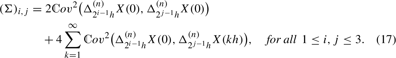
(16)
\[ \sqrt{N}\big({J_{N}}-\Psi (\Theta )\big)\stackrel{\mathcal{L}}{\longrightarrow }\mathcal{N}(0,\Sigma ),\hspace{1em}\textit{as}\hspace{2.5pt}N\to \infty ,\]Proof.
First, we recall that ${J_{l,N}}=\frac{1}{N}{\textstyle\sum _{k=0}^{N-1}}{({Z_{k}^{(l)}})^{2}}$, ${Z_{k}^{(l)}}={\Delta _{lh}^{(n)}}X(kh)$. Let  and set ${F_{N}}(\lambda )={\textstyle\sum _{j=1}^{3}}{\lambda _{j}}\{\sqrt{N}({J_{{2^{j-1}},N}}-{\Psi _{{2^{j-1}},n}}(\Theta ))\}$. Straightforward computations lead to
 . Since f is of Hermite rank 2 (see Lemma 3 in the Appendix), and because of stationarity of the sequence ${\{{Z_{k}}\}_{k=0}^{\infty }}$, we need only to examine the asymptotics of the covariance functions
In (18)–(19) we used the stationarity of increments of W and the fact that ${Y_{lh,r}^{(n)}}$ are independent of ${B_{H}^{n}}$, while (20) is justified by Lemma 4 in the Appendix. It follows that
provided that $H\lt n-1/4$. Similarly, we have ${\textstyle\sum _{k=-\infty }^{-1}}{\mathcal{R}^{i,j}}{(k)^{2}}\lt \infty $. Hence, by [2, Theorem 4] one has ${F_{N}}(\lambda )\stackrel{\mathcal{L}}{\longrightarrow }\mathcal{N}(0,{\sigma ^{2}}(\lambda ))$, as $N\to \infty $, with
. Since f is of Hermite rank 2 (see Lemma 3 in the Appendix), and because of stationarity of the sequence ${\{{Z_{k}}\}_{k=0}^{\infty }}$, we need only to examine the asymptotics of the covariance functions
In (18)–(19) we used the stationarity of increments of W and the fact that ${Y_{lh,r}^{(n)}}$ are independent of ${B_{H}^{n}}$, while (20) is justified by Lemma 4 in the Appendix. It follows that
provided that $H\lt n-1/4$. Similarly, we have ${\textstyle\sum _{k=-\infty }^{-1}}{\mathcal{R}^{i,j}}{(k)^{2}}\lt \infty $. Hence, by [2, Theorem 4] one has ${F_{N}}(\lambda )\stackrel{\mathcal{L}}{\longrightarrow }\mathcal{N}(0,{\sigma ^{2}}(\lambda ))$, as $N\to \infty $, with 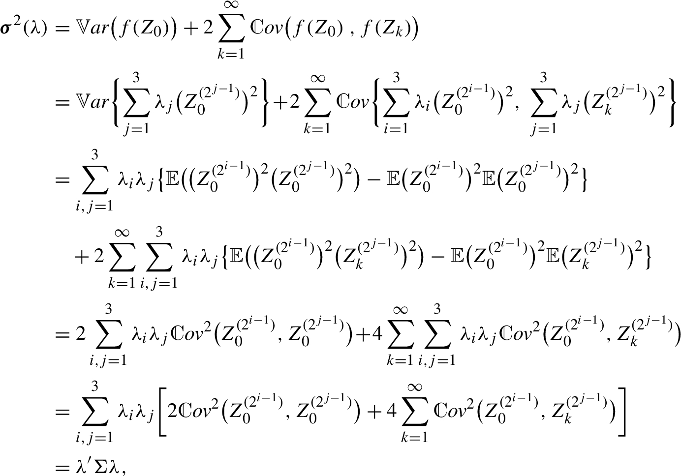
\[\begin{aligned}{}{F_{N}}(\lambda )& ={\sum \limits_{j=1}^{3}}{\lambda _{j}}\Bigg\{\sqrt{N}\Bigg(\frac{1}{N}{\sum \limits_{k=0}^{N-1}}{\big({Z_{k}^{({2^{j-1}})}}\big)^{2}}-{\Psi _{{2^{j-1}},n}}(\Theta )\Bigg)\Bigg\}\\ {} & =\frac{1}{\sqrt{N}}{\sum \limits_{k=0}^{N-1}}{\sum \limits_{j=1}^{3}}{\lambda _{j}}\big\{{\big({Z_{k}^{({2^{j-1}})}}\big)^{2}}-\mathbb{E}{\big({Z_{k}^{({2^{j-1}})}}\big)^{2}}\big\}\\ {} & =:\frac{1}{\sqrt{N}}{\sum \limits_{k=0}^{N-1}}\big\{f({Z_{k}})-\mathbb{E}f({Z_{k}})\big\},\hspace{1em}{Z_{k}}=\big({Z_{k}^{(1)}},{Z_{k}^{(2)}},{Z_{k}^{(4)}}\big),\end{aligned}\]
where $f(x,y,z)={\lambda _{1}}{x^{2}}+{\lambda _{2}}{y^{2}}+{\lambda _{3}}{z^{2}}$. According to the Cramér–Wold device, the vector $\sqrt{N}({J_{N}}-\Psi (\Theta ))$ is asymptotically normal if and only if ${F_{N}}(\lambda )$ is asymptotically normal for each
\[ {\mathcal{R}^{i,j}}(k):=\mathbb{E}\big({Z_{m}^{({2^{i-1}})}}{Z_{m+k}^{({2^{j-1}})}}\big)=\mathbb{E}\big({Z_{0}^{({2^{i-1}})}}{Z_{k}^{({2^{j-1}})}}\big),\hspace{1em}1\le i,j\le 3.\]
In fact, we shall prove that ${\textstyle\sum _{k=-\infty }^{\infty }}{\mathcal{R}^{i,j}}{(k)^{2}}\lt \infty $ for each i, j. Set $l={2^{i-1}}$, $p={2^{j-1}}$. We have (18)
\[\begin{aligned}{}& {\mathcal{R}^{i,j}}(k)\\ {} & \hspace{1em}=\mathbb{E}\big({\Delta _{lh}^{(n)}}X(0){\Delta _{ph}^{(n)}}X(kh)\big)\\ {} & \hspace{1em}={\alpha ^{2}}{\sum \limits_{{r_{1}}{r_{2}}=0}^{n-1}}{d_{{r_{1}}}^{(n-1)}}{d_{{r_{2}}}^{(n-1)}}\mathbb{E}\big({Y_{lh,{r_{1}}}^{(n)}}(0){Y_{ph,{r_{2}}}^{(n)}}(kh)\big)+{\sigma ^{2}}\mathbb{E}\big({\Delta _{lh}^{(n)}}{B_{H}^{n}}(0){\Delta _{ph}^{(n)}}{B_{H}^{n}}(kh)\big)\end{aligned}\](21)
\[ {\sum \limits_{k=1}^{\infty }}{\mathcal{R}^{i,j}}{(k)^{2}}\sim {\mathcal{C}_{H}^{(n)}}{(l,h)^{2}}{h^{4H-4n}}{\sum \limits_{k=1}^{\infty }}{k^{4H-4n}}\lt \infty ,\]where Σ is defined by (17). In the fourth equality above we used the fact that for any centered Gaussian vector $(\xi ,\zeta )$, we have  . It is not hard to see that
\[ \mathbb{E}{e^{i{\lambda ^{\prime }}\{\sqrt{N}({J_{N}}-\Psi (\Theta ))\}}}=\mathbb{E}{e^{i{F_{N}}(\lambda )}}\longrightarrow {e^{-\frac{1}{2}{\lambda ^{\prime }}\Sigma \lambda }},\hspace{1em}i=\sqrt{-1},\]
which completes the proof of (16). □Now, we are ready to apply the Delta method with the use of (16) to get the joint asymptotic normality of the estimators $\widehat{H}$, $\widehat{{\alpha ^{2}}}$ and $\widehat{{\sigma ^{2}}}$.
Theorem 3.
Consider $\widehat{\Theta }$, the estimator of $\Theta ={(H,{\alpha ^{2}},{\sigma ^{2}})^{\prime }}$ defined by (9)–(11), and let $H\in (n-1,n-1/4)$. Then we have $\sqrt{N}(\widehat{\Theta }-\Theta )\stackrel{\mathcal{L}}{\longrightarrow }\mathcal{N}(0,({D_{\Psi }^{-1}})\Sigma {({D_{\Psi }^{-1}})^{\prime }})$ where ${D_{\Psi }^{-1}}$ denotes the inverse of the Jacobian matrix
\[\begin{aligned}{}{D_{\Psi }}& =\left(\begin{array}{c}{\partial _{H}}{\Psi _{1,n}}(\Theta )\hspace{2.5pt}\hspace{2.5pt}\hspace{2.5pt}\hspace{2.5pt}{\partial _{{\alpha ^{2}}}}{\Psi _{1,n}}(\Theta )\hspace{2.5pt}\hspace{2.5pt}\hspace{2.5pt}\hspace{2.5pt}{\partial _{{\sigma ^{2}}}}{\Psi _{1,n}}(\Theta )\\ {} {\partial _{H}}{\Psi _{2,n}}(\Theta )\hspace{2.5pt}\hspace{2.5pt}\hspace{2.5pt}\hspace{2.5pt}{\partial _{{\alpha ^{2}}}}{\Psi _{2,n}}(\Theta )\hspace{2.5pt}\hspace{2.5pt}\hspace{2.5pt}\hspace{2.5pt}{\partial _{{\sigma ^{2}}}}{\Psi _{2,n}}(\Theta )\\ {} {\partial _{H}}{\Psi _{4,n}}(\Theta )\hspace{2.5pt}\hspace{2.5pt}\hspace{2.5pt}\hspace{2.5pt}{\partial _{{\alpha ^{2}}}}{\Psi _{4,n}}(\Theta )\hspace{2.5pt}\hspace{2.5pt}\hspace{2.5pt}\hspace{2.5pt}{\partial _{{\sigma ^{2}}}}{\Psi _{4,n}}(\Theta )\end{array}\right)\\ {} & =\left(\begin{array}{c@{\hskip10.0pt}c@{\hskip10.0pt}c}{\sigma ^{2}}{U^{\prime }_{H}}& V& {U_{H}}\\ {} {\sigma ^{2}}{2^{2H}}(2\log (2){U_{H}}+{U^{\prime }_{H}})& 2V& {2^{2H}}{U_{H}}\\ {} {\sigma ^{2}}{4^{2H}}(2\log (4){U_{H}}+{U^{\prime }_{H}})& 4V& {4^{2H}}{U_{H}}\end{array}\right),\end{aligned}\]
where ${U^{\prime }_{H}}={\partial _{H}}{U_{H}}$ with V, ${U_{H}}$ and ${\Psi _{l,n}}(\Theta )$, $l\gt 0$, being defined by (13)–(15).
Proof.
First, observe that $\widehat{\Theta }$ is constructed by solving the equation ${J_{N}}=\Psi (\widehat{\Theta })$, that is, $\widehat{\Theta }={\Psi ^{-1}}({J_{N}})$. To get the asymptotic normality of $\widehat{\Theta }$, it suffices to apply the Delta method to ${J_{N}}$ with the function ${\Psi ^{-1}}$. If ${D_{{\Psi ^{-1}}}}$, the Jacobian matrix of ${\Psi ^{-1}}$, exists then by [31, Theorem 3.1] we have $\sqrt{N}(\widehat{\Theta }-\Theta )\stackrel{\mathcal{L}}{\longrightarrow }{D_{{\Psi ^{-1}}}}\mathcal{N}(0,\Sigma )=\mathcal{N}(0,({D_{\Psi }^{-1}})\Sigma {({D_{\Psi }^{-1}})^{\prime }})$. Note that ${D_{{\Psi ^{-1}}}}$ exists if ${D_{\Psi }}$ is invertible. Evaluating the determinant of ${D_{\Psi }}$ gives
\[\begin{aligned}{}|{D_{\Psi }}|& =\left|\begin{array}{c@{\hskip10.0pt}c@{\hskip10.0pt}c}{\sigma ^{2}}{U^{\prime }_{H}}& V& {U_{H}}\\ {} {\sigma ^{2}}{2^{2H}}(2\log (2){U_{H}}+{U^{\prime }_{H}})& 2V& {2^{2H}}{U_{H}}\\ {} {\sigma ^{2}}{4^{2H}}(2\log (4){U_{H}}+{U^{\prime }_{H}})& 4V& {4^{2H}}{U_{H}}\end{array}\right|\\ {} & =V{\sigma ^{2}}{U_{H}}\left|\begin{array}{c@{\hskip10.0pt}c@{\hskip10.0pt}c}{U^{\prime }_{H}}& 1& 1\\ {} {2^{2H}}(2\log (2){U_{H}}+{U^{\prime }_{H}})& 2& {2^{2H}}\\ {} {4^{2H}}(4\log (2){U_{H}}+{U^{\prime }_{H}})& 4& {4^{2H}}\end{array}\right|\\ {} & =V{\sigma ^{2}}{U_{H}}\left|\begin{array}{c@{\hskip10.0pt}c@{\hskip10.0pt}c}{U^{\prime }_{H}}& 1& 1\\ {} \log (2){2^{2H+1}}{U_{H}}+({2^{2H}}-2){U^{\prime }_{H}}& 0& ({2^{2H}}-2)\\ {} \log (2){2^{4H+2}}{U_{H}}+({2^{4H}}-4){U^{\prime }_{H}}& 0& ({2^{4H}}-4)\end{array}\right|\\ {} & =-V{\sigma ^{2}}{U_{H}}\big({2^{2H}}-2\big)\left|\begin{array}{c@{\hskip10.0pt}c}\log (2){2^{2H+1}}{U_{H}}+({2^{2H}}-2){U^{\prime }_{H}}& 1\\ {} \log (2){2^{4H+2}}{U_{H}}+({2^{4H}}-4){U^{\prime }_{H}}& ({2^{2H}}+2)\end{array}\right|\\ {} & =-V{\sigma ^{2}}{U_{H}}\big({2^{2H}}-2\big)\big\{\log (2){2^{2H+1}}\big({2^{2H}}+2\big){U_{H}}-\log (2){2^{4H+2}}{U_{H}}\big\}\\ {} & =V{\sigma ^{2}}{U_{H}^{2}}\log (2){2^{2H+1}}{\big({2^{2H}}-2\big)^{2}}\gt 0.\end{aligned}\]
Hence, ${D_{\Psi }}$ is invertible and the proof is complete. □3.2 Estimating the drift parameter θ
The approach used in Subsection 3.1 to estimate H, ${\alpha ^{2}}$ and ${\sigma ^{2}}$ is suitable for the model (1) with no restrictions on $d(\mathcal{P})$, the degree of $\mathcal{P}$. Albeit, the drift parameter θ should be estimated differently, because taking higher increments cancels out the drift term. In the case where $d(\mathcal{P})\ge n$, we may readily estimate θ by ${\widetilde{\theta }_{t}}:=\frac{X(t)}{\mathcal{P}(t)}$, which satisfies the usual properties. But if $d(\mathcal{P})\lt n$ this estimator becomes inconsistent under $\mathbb{P}$. Assume that the parameters H, ${\alpha ^{2}}$ and ${\sigma ^{2}}$ are known (or previously estimated) with $\alpha \gt 0$, and let ${\mathbb{P}_{0}}$ be the probability measure under which W is a Wiener process independent of ${B_{H}^{n}}$. Then the following results are obtained.
Proposition 1.
The maximum likelihood estimator (MLE) of θ is given by
where ${M_{t}}={\mathbb{E}_{0}}({\textstyle\int _{0}^{t}}{\mathcal{P}^{\prime }}(s)dW(s)\mid {\mathcal{F}_{t}^{X}})$ is a Gaussian martingale with quadratic variation ${\langle M\rangle _{t}}={\mathbb{E}_{0}}({M_{t}^{2}})$.
Proof.
We proceed as in [4, 23] and construct the right likelihood function. In the first stage we rewrite (1) as $X(t)=\alpha \overline{W}(t)+\sigma {B_{H}^{n}}(t)$ with $W(t)=\overline{W}(t)-\frac{\theta }{\alpha }\mathcal{P}(t)$, where $\overline{W}$ is a Wiener process under ${\mathbb{P}_{\theta }}$. Here, ${\mathbb{P}_{\theta }}$ is the probability measure under which $\overline{W}$ and ${B_{H}^{n}}$ are independent. Clearly, ${\mathbb{P}_{\theta }}\ll {\mathbb{P}_{0}}$, where ${\mathbb{P}_{0}}$ corresponds to the case when $\theta =0$. The corresponding Radon–Nikodym derivative is given by
where ${\zeta _{t}}={\textstyle\int _{0}^{t}}{\mathcal{P}^{\prime }}(s)dW(s)$ with its quadratic variation ${\langle \zeta \rangle _{t}}$, ${M_{T}}={\mathbb{E}_{0}}({\zeta _{T}}\mid {\mathcal{F}_{T}^{X}})$ and ${V_{T}}={\mathbb{E}_{0}}({({M_{T}}-{\zeta _{T}})^{2}}\mid {\mathcal{F}_{T}^{X}})$. In (23) we used the fact that $\overline{W}$ coincides with W under ${\mathbb{P}_{0}}$, while (24) is due to the Gaussian nature of ${\zeta _{T}}$ given ${\mathcal{F}_{t}^{X}}$ with mean ${M_{T}}$ and variance ${V_{T}}$. It is worth to mention that ${L_{T}}(X,\theta )$ is the Radon–Nikodym derivative of ${\mu _{\theta }}$ with respect to ${\mu _{0}}$, where ${\mu _{\theta }}$ is the probability induced by X on the space of continuous functions with the usual supremum topology under probability ${\mathbb{P}_{\theta }}$.
\[ \frac{d{\mathbb{P}_{\theta }}}{d{\mathbb{P}_{0}}}=\exp \Bigg(\frac{\theta }{\alpha }{\int _{0}^{T}}{\mathcal{P}^{\prime }}(s)d\overline{W}(s)-\frac{{\theta ^{2}}}{2{\alpha ^{2}}}{\int _{0}^{T}}{\mathcal{P}^{\prime }}{(s)^{2}}ds\Bigg)\]
and is justified by the Girsanov theorem. But it is not the likelihood of (1) unless ${\mathcal{F}_{t}^{\overline{W}}}={\mathcal{F}_{t}^{X}}$, otherwise, we shall consider its conditional expectation (23)
\[\begin{array}{r@{\hskip0pt}l@{\hskip0pt}r}\displaystyle {L_{T}}(X,\theta )& \displaystyle ={\mathbb{E}_{0}}\bigg(\frac{d{\mathbb{P}_{\theta }}}{d{\mathbb{P}_{0}}}\mid {\mathcal{F}_{T}^{X}}\bigg)\hspace{2em}\\ {} & \displaystyle ={\mathbb{E}_{0}}\Bigg\{\exp \Bigg(\frac{\theta }{\alpha }{\int _{0}^{T}}{\mathcal{P}^{\prime }}(s)d\overline{W}(s)-\frac{{\theta ^{2}}}{2{\alpha ^{2}}}{\int _{0}^{T}}{\mathcal{P}^{\prime }}{(s)^{2}}ds\Bigg)\mid {\mathcal{F}_{T}^{X}}\Bigg\}\hspace{2em}\\ {} & \displaystyle ={\mathbb{E}_{0}}\Bigg\{\exp \Bigg(\frac{\theta }{\alpha }{\int _{0}^{T}}{\mathcal{P}^{\prime }}(s)dW(s)-\frac{{\theta ^{2}}}{2{\alpha ^{2}}}{\int _{0}^{T}}{\mathcal{P}^{\prime }}{(s)^{2}}ds\Bigg)\mid {\mathcal{F}_{T}^{X}}\Bigg\}\hspace{2em}& \hspace{2.5pt}\end{array}\](24)
\[\begin{aligned}{}& =\exp \bigg(-\frac{{\theta ^{2}}}{2{\alpha ^{2}}}{\langle \zeta \rangle _{T}}\bigg){\mathbb{E}_{0}}\bigg\{\exp \bigg(\frac{\theta }{\alpha }{\zeta _{T}}\bigg)\mid {\mathcal{F}_{T}^{X}}\bigg\}\hspace{2em}\\ {} & =\exp \bigg(\frac{\theta }{\alpha }{M_{T}}-\frac{{\theta ^{2}}}{2{\alpha ^{2}}}\big({\langle \zeta \rangle _{T}}-{V_{T}}\big)\bigg),\hspace{2em}\end{aligned}\]Since M is an ${\mathcal{F}_{t}^{X}}$-measurable Gaussian martingale, then its quadratic variation $\langle M\rangle $ is deterministic and one has
As a result, we have the martingale property:
On the other hand, for all $t\gt s$
We used ${V_{t}}={\mathbb{E}_{0}}({\zeta _{t}^{2}}\mid {\mathcal{F}_{t}^{X}})-{M_{t}^{2}}$ in the first equality above, while the third equality follows by the martingale property of $({\zeta _{t}},{\mathcal{F}_{t}})$. Combining (26)–(27) with (25) we can assert that ${\langle M\rangle _{t}}={\langle \zeta \rangle _{t}}-{\mathbb{E}_{0}}{({M_{t}}-{\zeta _{t}})^{2}}={\langle \zeta \rangle _{t}}-{V_{t}}$. Hence, (24) becomes
(25)
\[\begin{aligned}{}{\langle M\rangle _{t}}& ={\mathbb{E}_{0}}\big({M_{t}^{2}}\big)={\mathbb{E}_{0}}\big({M_{t}}{\mathbb{E}_{0}}\big({\zeta _{t}}\mid {\mathcal{F}_{t}^{X}}\big)\big)={\mathbb{E}_{0}}({M_{t}}{\zeta _{t}})\\ {} & =\frac{1}{2}{\mathbb{E}_{0}}\big\{{M_{t}^{2}}+{\zeta _{t}^{2}}-{({M_{t}}-{\zeta _{t}})^{2}}\big\}\\ {} & ={\mathbb{E}_{0}}\big({\zeta _{t}^{2}}\big)-{\mathbb{E}_{0}}{({M_{t}}-{\zeta _{t}})^{2}}\\ {} & ={\langle \zeta \rangle _{t}}-{\mathbb{E}_{0}}{({M_{t}}-{\zeta _{t}})^{2}}.\end{aligned}\](26)
\[ {\mathbb{E}_{0}}\big\{{M_{t}^{2}}-\big[{\langle \zeta \rangle _{t}}-{\mathbb{E}_{0}}{({M_{t}}-{\zeta _{t}})^{2}}\big]\mid {\mathcal{F}_{s}^{X}}\big\}={M_{s}^{2}}-\big[{\langle \zeta \rangle _{s}}-{\mathbb{E}_{0}}{({M_{s}}-{\zeta _{s}})^{2}}\big],\hspace{1em}\forall t\gt s.\](27)
\[\begin{aligned}{}& {\mathbb{E}_{0}}\big\{{M_{t}^{2}}-\big[{\langle \zeta \rangle _{t}}-{V_{t}}\big]\mid {\mathcal{F}_{s}^{X}}\big\}={\mathbb{E}_{0}}\big\{{\mathbb{E}_{0}}\big({\zeta _{t}^{2}}-{\langle \zeta \rangle _{t}}\mid {\mathcal{F}_{t}^{X}}\big)\mid {\mathcal{F}_{s}^{X}}\big\}\\ {} & \hspace{1em}={\mathbb{E}_{0}}\big\{{\mathbb{E}_{0}}\big({\zeta _{t}^{2}}-{\langle \zeta \rangle _{t}}\mid {\mathcal{F}_{s}}\big)\mid {\mathcal{F}_{s}^{X}}\big\},\hspace{2.5pt}\big({\mathcal{F}_{s}^{X}}\subset {\mathcal{F}_{t}^{X}}\hspace{2.5pt}\text{and}\hspace{2.5pt}{\mathcal{F}_{s}^{X}}\subset {\mathcal{F}_{s}}\big)\\ {} & \hspace{1em}={\mathbb{E}_{0}}\big({\zeta _{s}^{2}}-{\langle \zeta \rangle _{s}}\mid {\mathcal{F}_{s}^{X}}\big)={\mathbb{E}_{0}}\big({\zeta _{s}^{2}}\mid {\mathcal{F}_{s}^{X}}\big)-{\langle \zeta \rangle _{s}}\\ {} & \hspace{1em}={M_{s}^{2}}-\big[{\langle \zeta \rangle _{s}}+{M_{s}^{2}}-{\mathbb{E}_{0}}\big({\zeta _{s}^{2}}\mid {\mathcal{F}_{s}^{X}}\big)\big]={M_{s}^{2}}-\big[{\langle \zeta \rangle _{s}}-{V_{s}}\big].\end{aligned}\]This expression of the likelihood at hand allows us to define the MLE of θ as ${\widehat{\theta }_{T}}=\alpha \frac{{M_{T}}}{{\langle M\rangle _{T}}}$. Hence, the proof is complete. □
Proposition 2.
The estimator ${\widehat{\theta }_{T}}$ defined by (22) can be rewritten as
where the kernel $K(\cdot ,\cdot )$ is defined by $K(T,s)=\frac{1}{T}{g_{T}}(\frac{s}{T})$, for all $s\in [0,T]$ with
Here ${({\gamma _{j}},\hspace{2.5pt}{\psi _{j}})_{j=0}^{\infty }}$ denotes the system of eigenvalues and eigenvectors of the integral operator with the kernel ${G_{H-1,n-1}}$ defined by formula (3).
(28)
\[ {\widehat{\theta }_{T}}=\frac{{\textstyle\textstyle\int _{0}^{T}}K(T,s)dX(s)}{{\textstyle\textstyle\int _{0}^{T}}K(T,s){\mathcal{P}^{\prime }}(s)ds},\]Proof.
Under ${\mathbb{P}_{\theta }}$, the model (1) can be rewritten as $X(t)=\sigma {\textstyle\int _{0}^{t}}{B_{H-1}^{n-1}}(s)ds+{\textstyle\int _{0}^{t}}\alpha d\overline{W}(s)$, for all $t\in [0,T]$. Set ${\overline{\zeta }_{T}}={\textstyle\int _{0}^{T}}{\mathcal{P}^{\prime }}(s)d\overline{W}(s)$. It is not hard to see that $({\overline{\zeta }_{T}},X(t))$ forms a Gaussian system, thus we can assert that (e.g., [20, Lemma 10.1]) for each $t\in [0,T]$ there is a function $s\mapsto K(t,s)$ defined on $[0,t]$ such that
Note that we used the fact that $\overline{W}=W$ under ${\mathbb{P}_{0}}$. We know also that
\[ {\mathbb{E}_{\theta }}\big({\overline{\zeta }_{T}}\mid {\mathcal{F}_{t}^{X}}\big)={\int _{0}^{t}}K(t,s)dX(s),\hspace{1em}{\mathbb{P}_{\theta }}\text{-a.s.}\]
In particular,
(31)
\[ {M_{T}}={\mathbb{E}_{0}}\big({\zeta _{T}}\mid {\mathcal{F}_{T}^{X}}\big)={\int _{0}^{T}}K(T,s)dX(s),\hspace{1em}{\mathbb{P}_{0}}\text{-a.s.}\]
\[\begin{aligned}{}{\langle M\rangle _{T}}& ={\mathbb{E}_{0}}\big({M_{T}^{2}}\big)={\mathbb{E}_{0}}({M_{T}}{\zeta _{T}})\\ {} & ={\mathbb{E}_{0}}\Bigg\{{\int _{0}^{T}}{\mathcal{P}^{\prime }}(s)dW(s)\Bigg(\alpha {\int _{0}^{T}}K(T,s)dW(s)+\sigma {\int _{0}^{T}}K(T,s)d{B_{H}^{n}}(s)\Bigg)\Bigg\}\\ {} & =\alpha {\int _{0}^{T}}K(T,s){\mathcal{P}^{\prime }}(s)ds.\end{aligned}\]
It follows that
To complete the proof we shall justify equations (29)–(30). First, observe that under ${\mathbb{P}_{0}}$ we have
for all $s\in [0,1]$. We will construct a solution ${g_{T}}(\cdot )$ to this equation. As the kernel ${G_{H-1,n-1}}$ is continuous symmetric and positive on $[0,1]\times [0,1]$, it follows by Mercer’s theorem (e.g., [13, p. 136]) that for all $s,u\in [0,1]$
\[\begin{aligned}{}dX(t)& =\alpha d\overline{W}(t)+\sigma d{B_{H}^{n}}(t)\\ {} & =\alpha dW(t)+\sigma {B_{H-1}^{n-1}}(t)dt.\end{aligned}\]
Second, by definition ${M_{T}}$ must satisfy the equation ${\mathbb{E}_{0}}(X(s){\zeta _{T}})={\mathbb{E}_{0}}(X(s){M_{T}})$, for all $s\in [0,T]$, which becomes, after some computations,
\[ \alpha {\int _{0}^{s}}{\mathcal{P}^{\prime }}(u)du={\alpha ^{2}}{\int _{0}^{s}}K(T,u)du+{\sigma ^{2}}{\int _{0}^{T}}{\int _{0}^{s}}K(T,u){G_{H-1,n-1}}(u,v)dvdu.\]
Differentiating this equation with respect to the variable s yields
\[ \alpha {\mathcal{P}^{\prime }}(s)={\alpha ^{2}}K(T,s)+{\sigma ^{2}}{\int _{0}^{T}}K(T,u){G_{H-1,n-1}}(u,s)du\]
for all $s\in [0,T]$. Set ${g_{T}}(s)=TK(T,Ts)$. After the change of variables $v=u/T$ and substituting s by $Ts$ we get
(33)
\[\begin{aligned}{}{\varphi _{T}}(s)& ={g_{T}}(s)+{\lambda ^{2}}{\int _{0}^{1}}{g_{T}}(u){\overline{G}_{T}}(s,u)du\hspace{1em}(\lambda =\sigma /\alpha ),\\ {} {\overline{G}_{T}}(s,u)& ={T^{2H-1}}{G_{H-1,n-1}}(u,s),\hspace{1em}{\varphi _{T}}(s)=\frac{T}{\alpha }{\mathcal{P}^{\prime }}(Ts),\end{aligned}\]
\[ {\overline{G}_{T}}(s,u)={T^{2H-1}}\sum \limits_{j\ge 0}{\gamma _{j}}{\psi _{j}}(s){\psi _{j}}(u),\]
with ${({\gamma _{j}},\hspace{2.5pt}{\psi _{j}})_{j=0}^{\infty }}$ being the system of eigenvalues and eigenvectors of the integral operator defined on ${L^{2}}([0,1])$ by
where ${({\psi _{j}})_{j=0}^{\infty }}$ forms an orthonormal basis of ${L^{2}}([0,1])$ and ${\{{\gamma _{j}}\}_{j=0}^{\infty }}\downarrow 0$. A solution to (33) of the form $y(s)={\varphi _{T}}(s)+{\textstyle\sum _{j\ge 0}}{a_{j}}{\psi _{j}}(s)$ exists if and only if
\[ \sum \limits_{j\ge 0}{\psi _{j}}(s)\Bigg[{a_{j}}+{\lambda ^{2}}{T^{2H-1}}{\gamma _{j}}\Bigg({\int _{0}^{1}}{\varphi _{T}}(u){\psi _{j}}(u)du+\sum \limits_{l\ge 0}{a_{l}}{\int _{0}^{1}}{\psi _{l}}(u){\psi _{j}}(u)du\Bigg)\Bigg]=0.\]
Identifying the coefficients we get, for each $j\ge 0$,
and the proof is then complete. □Theorem 4.
Proof.
Taking expectations in both sides of (32) and observing that ${\langle M\rangle _{T}}$ is deterministic we obtain
\[\begin{aligned}{}{\mathbb{E}_{\theta }}({\widehat{\theta }_{T}})& ={\mathbb{E}_{\theta }}\bigg(\alpha \frac{{M_{T}}}{{\langle M\rangle _{T}}}\bigg)=\frac{\alpha }{{\langle M\rangle _{T}}}{\mathbb{E}_{0}}\big({M_{T}}{L_{T}}(X,\theta )\big)\\ {} & =\frac{\alpha }{{\langle M\rangle _{T}}}{\mathbb{E}_{0}}\big({M_{T}}{e^{\frac{\theta }{\alpha }{M_{T}}-\frac{{\theta ^{2}}}{2{\alpha ^{2}}}{\langle M\rangle _{T}}}}\big)\\ {} & =\frac{\alpha }{{\langle M\rangle _{T}}}{e^{-\frac{{\theta ^{2}}}{2{\alpha ^{2}}}{\langle M\rangle _{T}}}}{\mathbb{E}_{0}}\bigg(\alpha \frac{d}{d\theta }\big({e^{\frac{\theta }{\alpha }{M_{T}}}}\big)\bigg)\\ {} & =\frac{{\alpha ^{2}}}{{\langle M\rangle _{T}}}{e^{-\frac{{\theta ^{2}}}{2{\alpha ^{2}}}{\langle M\rangle _{T}}}}\frac{d}{d\theta }\big\{{e^{\frac{{\theta ^{2}}}{2{\alpha ^{2}}}{\langle M\rangle _{T}}}}{\mathbb{E}_{0}}\big({L_{T}}(X,\theta )\big)\big\}=\theta .\end{aligned}\]
Similarly, we have
\[\begin{aligned}{}{\mathbb{E}_{\theta }}\big({\widehat{\theta }_{T}^{2}}\big)& =\frac{{\alpha ^{2}}}{{\langle M\rangle _{T}^{2}}}{\mathbb{E}_{0}}\big({M_{T}^{2}}{L_{T}}(X,\theta )\big)\\ {} & =\frac{{\alpha ^{2}}}{{\langle M\rangle _{T}^{2}}}{\mathbb{E}_{0}}\big({M_{T}^{2}}{e^{\frac{\theta }{\alpha }{M_{T}}-\frac{{\theta ^{2}}}{2{\alpha ^{2}}}{\langle M\rangle _{T}}}}\big)\\ {} & =\frac{{\alpha ^{2}}}{{\langle M\rangle _{T}^{2}}}{e^{-\frac{{\theta ^{2}}}{2{\alpha ^{2}}}{\langle M\rangle _{T}}}}{\mathbb{E}_{0}}\bigg({\alpha ^{2}}\frac{{d^{2}}}{d{\theta ^{2}}}\big({e^{\frac{\theta }{\alpha }{M_{T}}}}\big)\bigg)\\ {} & =\frac{{\alpha ^{4}}}{{\langle M\rangle _{T}^{2}}}{e^{-\frac{{\theta ^{2}}}{2{\alpha ^{2}}}{\langle M\rangle _{T}}}}\frac{{d^{2}}}{d{\theta ^{2}}}\big\{{e^{\frac{{\theta ^{2}}}{2{\alpha ^{2}}}{\langle M\rangle _{T}}}}{\mathbb{E}_{0}}\big({L_{T}}(X,\theta )\big)\big\}\\ {} & =\frac{{\alpha ^{2}}}{{\langle M\rangle _{T}}}+{\theta ^{2}}.\end{aligned}\]
Hence, $\mathbb{V}\mathit{ar}({\widehat{\theta }_{T}})={\alpha ^{2}}/{\langle M\rangle _{T}}$ and by Gaussianity of ${\widehat{\theta }_{T}}$ the last statement follows. There remains to show that ${\langle M\rangle _{T}}\longrightarrow \infty $ as $T\to \infty $. Let d be the degree of $\mathcal{P}$. By virtue of the self-similarity of W and the change of variables $u=s/T$ one has
\[\begin{aligned}{}{M_{T}}& ={\mathbb{E}_{0}}\big({\zeta _{T}}\mid {\mathcal{F}_{T}^{X}}\big)={\mathbb{E}_{0}}\Bigg({\int _{0}^{T}}{\mathcal{P}^{\prime }}(s)dW(s)\mid {\mathcal{F}_{T}^{X}}\Bigg)\\ {} & ={T^{1/2}}{\mathbb{E}_{0}}\Bigg({\int _{0}^{1}}{\mathcal{P}^{\prime }}(Tu)dW(u)\mid {\mathcal{F}_{T}^{X}}\Bigg)\\ {} & ={T^{1/2}}{\sum \limits_{j=1}^{d}}(j{a_{j}}){T^{j-1}}{\mathbb{E}_{0}}\Bigg({\int _{0}^{1}}{u^{j-1}}dW(u)\mid {\mathcal{F}_{T}^{X}}\Bigg)\\ {} & =:{T^{1/2}}{\sum \limits_{j=1}^{d}}(j{a_{j}}){T^{j-1}}{A_{j,T}}.\end{aligned}\]
Let ${\{{T_{k}}\}_{k=1}^{\infty }}\uparrow \infty $ be a sequence of nonnegative numbers and set ${\xi _{k}}={T_{k}^{1/2-d}}{M_{{T_{k}}}}$. Clearly, ${\mathcal{F}_{\infty }^{X}}=\sigma ({\textstyle\bigcup _{t\ge 0}}{\mathcal{F}_{t}^{X}})=\sigma ({\textstyle\bigcup _{k=1}^{\infty }}{\mathcal{F}_{{T_{k}}}^{X}})$ and ${\mathcal{F}_{{T_{1}}}^{X}}\subseteq {\mathcal{F}_{{T_{2}}}^{X}}\subseteq \cdots \mathcal{F}$. On the other hand, ${\mathbb{E}_{0}}|{\textstyle\int _{0}^{1}}{u^{j-1}}dW(u)|\le \sqrt{{\textstyle\int _{0}^{1}}{u^{2j-2}}du}\le 1$, for all $j=1,2,\dots ,d$. Therefore, for each j we have almost surely (e.g., [29, p. 510]) ${A_{j,{T_{k}}}}\longrightarrow {A_{j,\infty }}$ as $k\uparrow \infty $. So we deduce that ${\xi _{k}^{2}}\sim {(d{a_{d}}{A_{d,\infty }})^{2}}$, as $k\uparrow \infty $. One can readily verify that ${\sup _{k\ge 1}}{\mathbb{E}_{0}}({\xi _{k}^{4}})\lt \infty $, which guarantees the uniform integrability of ${\{{\xi _{k}^{2}}\}_{k}}$. Thus (e.g., [29, Theorem 4]) ${T_{k}^{1-2d}}{\langle M\rangle _{{T_{k}}}}={\mathbb{E}_{0}}({\xi _{k}^{2}})\longrightarrow {\mathbb{E}_{0}}{(d{a_{d}}{A_{d,\infty }})^{2}}$. Finally, by the arbitrariness of ${\{{T_{k}}\}_{k}}$ we conclude that ${\langle M\rangle _{T}}\sim {\mathbb{E}_{0}}{(d{a_{d}}{A_{d,\infty }})^{2}}{T^{2d-1}}$, as $T\to \infty $ with $d\in [1,n)$. □Corollary 1.
For any $\gamma \gt 1/(2d(\mathcal{P})-1)$ the estimator ${\widehat{\theta }_{{N^{\gamma }}}}$ is strongly consistent, where $d(\mathcal{P})$ is the degree of the polynomial function $\mathcal{P}$.
Proof.
While proving Theorem 4 we have shown that ${\mathbb{E}_{\theta }}{({\widehat{\theta }_{T}}-\theta )^{2}}={\alpha ^{2}}/{\langle M\rangle _{T}}$ and ${\langle M\rangle _{T}}\sim {\mathbb{E}_{0}}{(d{a_{d}}{A_{d,\infty }})^{2}}{T^{2d-1}}$, as $T\to \infty $, where
\[ {A_{d,\infty }}={\mathbb{E}_{0}}\Bigg({\int _{0}^{1}}{u^{d-1}}dW(u)\mid {\mathcal{F}_{\infty }^{X}}\Bigg)\]
and ${a_{d}}$ is the leading coefficient of the polynomial function $\mathcal{P}$ of degree $d=d(\mathcal{P})\in [1,n)$. Let $\epsilon \gt 0$ and set $T={N^{\gamma }}$. We have
\[\begin{aligned}{}\sum \limits_{N\ge 1}{\mathbb{P}_{\theta }}\big(|{\widehat{\theta }_{{N^{\gamma }}}}-\theta |\gt \epsilon \big)& \le {\epsilon ^{-2}}\sum \limits_{N\ge 1}{\mathbb{E}_{\theta }}{({\widehat{\theta }_{{N^{\gamma }}}}-\theta )^{2}}\\ {} & \le \sum \limits_{N\ge 1}\frac{{\alpha ^{2}}}{{\epsilon ^{2}}{\langle M\rangle _{{N^{\gamma }}}}}\sim C\sum \limits_{N\ge 1}{N^{\gamma (1-2d)}}\lt \infty ,\end{aligned}\]
provided that $\gamma \gt 1/(2d-1)$ and C is some nonnegative constant. By using the Borel–Cantelli lemma we can assert that Corollary 1 is well established. □4 Concluding remarks
In the present work an nth-order mixed fractional Brownian motion with polynomial drift was studied. Based on discrete observations, we constructed estimators $(\widehat{H},\widehat{{\alpha ^{2}}},\widehat{{\sigma ^{2}}})$ of the noise parameters $(H,{\alpha ^{2}},{\sigma ^{2}})$ and examined their asymptotic behavior (consistency and asymptotic normality) by taking higher order increments and using the ergodic theorem. We stress that taking higher order increments cancels out the drift. Thus, we estimated the drift parameter θ independently by using the maximum likelihood approach based on continuous obervations $\{X(t):t\in [0,T]\}$. Based on limiting distributions results with the use of Prohorov’s theorem, the estimators of ${\alpha ^{2}}$ and θ (with $T=N$ being the time horizon or number of observations) show the same performance as those given in [11]. They have the rate of convergence of order ${\mathcal{O}_{\mathbb{P}}}({N^{-1/2}})$ and ${\mathcal{O}_{\mathbb{P}}}({N^{1/2-d(\mathcal{P})}})$, respectively. Unlike [11] in which the estimator of ${\sigma ^{2}}$ has the rate of convergence of order ${\mathcal{O}_{\mathbb{P}}}({N^{1/2-H}})$, the rate of convergence established here equals ${\mathcal{O}_{\mathbb{P}}}({N^{-1/2}})$ and is of great importance when $H\in (0,1)$. The limiting distributions provided in [11] are nonnormal (except for the estimator of ${\alpha ^{2}}$), while those given here are all normal. This would simplify the task of finding the associated confidence intervals. An extension of this work would be to study a model driven by an infinite mixture of higher order fBm’s (see [9]).


